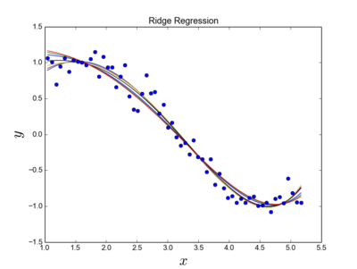
Linear Least-Squares L2-Regularized Regression System
A Linear Least-Squares L2-Regularized Regression System is an regularized linear regression system that implements a linear least-squares l2-regularized regression algorithm to solve a ridge regression task.
- AKA: Ridge Regression System, Tikhonov-Miller Regularized System, Phillips-Twomey Regression System, Constrained Linear Inversion System.
- Example(s)
sklearn.linear_model.Ridgea Scikit Learn mode that solves a regression model where the loss function is the linear least squares function and regularization is given by the l2-normExamples:
| Input: | Output: |
source code:
ridgeregression.py |

|
- Counter-Example(s):
- See: Support Vector Machine, Andrey Nikolayevich Tikhonov, Regularization (Mathematics), Ill-Posed Problem, Statistics, Machine Learning, Levenberg–Marquardt Algorithm, Non-Linear Least Squares, Ordinary Least Squares, Well-Posed Problem, Overdetermined System, Over-Fitted.
References
2017
- http://scikit-learn.org/stable/modules/generated/sklearn.linear_model.Ridge.html#sklearn.linear_model.Ridge
- QUOTE: Linear least squares with l2 regularization.
This model solves a regression model where the loss function is the linear least squares function and regularization is given by the l2-norm. Also known as Ridge Regression or Tikhonov regularization. This estimator has built-in support for multi-variate regression (i.e., when y is a 2d-array of shape [n_samples, n_targets]). (...)
Examples
- QUOTE: Linear least squares with l2 regularization.
| >>> from sklearn.linear_model import Ridge >>> import numpy as np >>> n_samples, n_features = 10, 5 >>> np.random.seed(0) >>> y = np.random.randn(n_samples) >>> X = np.random.randn(n_samples, n_features) >>> clf = Ridge(alpha=1.0) >>> clf.fit(X, y) Ridge(alpha=1.0, copy_X=True, fit_intercept=True, max_iter=None, normalize=False, random_state=None, solver='auto', tol=0.001) |
2016
- (Jain, 2016) Aarshay Jain (2016) ⇒ https://www.analyticsvidhya.com/blog/2016/01/complete-tutorial-ridge-lasso-regression-python/#three
- QUOTE: 3. Ridge Regression
As mentioned before, ridge regression performs ‘L2 regularization‘, i.e. it adds a factor of sum of squares of coefficients in the optimization objective. Thus, ridge regression optimizes the following:
Objective = RSS + α * (sum of square of coefficients)
Here, α (alpha) is the parameter which balances the amount of emphasis given to minimizing RSS vs minimizing sum of square of coefficients. α can take various values:
- α = 0:
- The objective becomes same as simple linear regression.
- We’ll get the same coefficients as simple linear regression.
- α = ∞:
- The coefficients will be zero. Why? Because of infinite weightage on square of coefficients, anything less than zero will make the objective infinite.
- 0 < α < ∞:
- The magnitude of α will decide the weightage given to different parts of objective.
- The coefficients will be somewhere between 0 and ones for simple linear regression.
I hope this gives some sense on how α would impact the magnitude of coefficients. One thing is for sure that any non-zero value would give values less than that of simple linear regression. By how much? We’ll find out soon. Leaving the mathematical details for later, lets see ridge regression in action on the same problem as above.
First, lets define a generic function for ridge regression similar to the one defined for simple linear regression. The Python code is:
- α = 0:
- QUOTE: 3. Ridge Regression
from sklearn.linear_model import Ridge
def ridge_regression(data, predictors, alpha, models_to_plot={}):
    #Fit the model
    ridgereg = Ridge(alpha=alpha,normalize=True)
    ridgereg.fit(data[predictors],data['y'])
    y_pred = ridgereg.predict(data[predictors])

    #Check if a plot is to be made for the entered alpha
    if alpha in models_to_plot:
        plt.subplot(models_to_plot[alpha])
        plt.tight_layout()
        plt.plot(data['x'],y_pred)
        plt.plot(data['x'],data['y'],'.')
        plt.title('Plot for alpha: %.3g'%alpha)

    #Return the result in pre-defined format
    rss = sum((y_pred-data['y'])**2)
    ret = [rss]
    ret.extend([ridgereg.intercept_])
    ret.extend(ridgereg.coef_)
    return ret