Variational Autoencoding (VAE) Algorithm
(Redirected from Variational Autoencoding Algorithm)
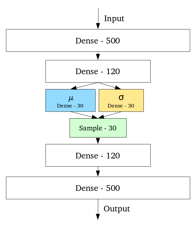
A Variational Autoencoding (VAE) Algorithm is an autoencoding algorithm (to train a VAE network) that assumes latent variable distributions from a Gaussian prior and utilizes a variational approach to approximate a latent space posterior distribution.
- Context:
- It can (often) can be implemented by an Variational Autoencoding System (that can solve an variational autoencoding training task to train an variational autoencoder).
- It can (often) use a Gaussian prior in the latent space to make variational inference tractable.
- ...
- It can range from being a Basic Variational Autoencoder to a more complex model like Vector Quantized-Variational Autoencoder (VQ-VAE).
- ...
- It can be implemented by a VAE System (that solves a VAE task) by learning latent variable representations from input data.
- It can utilize Variational Inference to approximate the posterior distribution over the latent space, minimizing the Kullback-Leibler divergence (KL divergence) between the true posterior and the variational approximation.
- It can rely on the Reparameterization Trick to enable efficient backpropagation through stochastic layers by transforming the sampling process into a differentiable function.
- It can employ a Stochastic Gradient Variational Bayes (SGVB) method to optimize the Evidence Lower Bound (ELBO), balancing reconstruction accuracy with latent space regularization.
- It can represent complex, high-dimensional data distributions, such as images, by learning a compact latent representation in the latent variable model.
- It can be used to interpolate between data points in the latent space, making it useful for generating synthetic samples or reconstructions.
- It can handle tasks like image generation, text generation, and data augmentation due to its generative capabilities.
- ...
- Example(s):
- Variational Autoencoder with an LSTM Decoder: an extension where the decoder is a Long Short-Term Memory (LSTM) network, useful for sequential data like text.
- Vector Quantized-Variational Autoencoder (VQ-VAE): a variant that quantizes the latent space, often used for high-quality image and video generation.
- Conditional Variational Autoencoder (CVAE): a variant conditioned on additional input data, making it useful for tasks like image-to-image translation.
- Beta-VAE: a variant that adds a parameter to control the balance between the KL divergence and reconstruction loss, often used to enforce disentanglement in the latent space.
- ...
- Counter-Example(s):
- Denoising Autoencoder: does not assume a probabilistic latent space and primarily focuses on learning to reconstruct inputs from noisy versions.
- Generative Adversarial Network (GAN): uses a different approach for generative modeling by pitting a generator against a discriminator, rather than relying on latent variable modeling.
- Autoregressive Transformer-based Model: generates sequences without latent variable modeling, focusing on autoregressive prediction.
- Principal Component Analysis (PCA): while also a dimensionality reduction technique, PCA is a linear model and does not use probabilistic inference or latent variable modeling.
- See: Variational Bayes, Generative Model, Autoencoder, Evidence Lower Bound (ELBO).
References
2024
- LLM
ALGORITHM VariationalAutoencoder:
   INPUT:
       - data: input data for training
       - latent_dim: dimension of the latent space
       - encoder: neural network mapping input data to latent space
       - decoder: neural network mapping latent space back to input space
       - learning_rate: rate for updating model weights
       - epochs: number of training iterations
   OUTPUT:
       - trained_encoder: trained encoder network
       - trained_decoder: trained decoder network
   // Initialize
   1. Initialize encoder and decoder neural networks
   2. Define the loss function as the sum of reconstruction loss and KL divergence
   3. Define the optimizer with the given learning_rate
   4. best_loss = infinity
   // Main training loop
   FOR epoch = 1 TO epochs:
       FOR each batch of data:
           // Encode the input data
           5. z_mean, z_log_var = ENCODE(encoder, batch)
           // Sample from the latent space using reparameterization trick
           6. z = z_mean + exp(0.5 * z_log_var) * epsilon
           // Decode the sampled latent variables
           7. reconstructed_data = DECODE(decoder, z)
           // Compute reconstruction loss
           8. recon_loss = MSE(reconstructed_data, batch)
           // Compute KL divergence
           9. kl_divergence = -0.5 * SUM(1 + z_log_var - z_mean^2 - exp(z_log_var))
           // Compute total loss
           10. total_loss = recon_loss + kl_divergence
           // Backpropagate the loss and update weights
           11. optimizer.zero_grad()
           12. total_loss.backward()
           13. optimizer.step()
       // Track the best model based on the loss
       14. IF total_loss < best_loss:
           15. best_loss = total_loss
           16. best_encoder = encoder
           17. best_decoder = decoder
RETURN best_encoder, best_decoder
FUNCTION ENCODE(encoder, data):
   // The encoder transforms the input data to latent mean and variance
   // Returns z_mean and z_log_var
FUNCTION DECODE(decoder, z):
   // The decoder transforms latent space variables back into data space
   // Returns reconstructed data
END ALGORITHM
2022
- (Wikipedia, 2022) ⇒ https://en.wikipedia.org/wiki/Variational_autoencoder Retrieved:2022-12-12.
- In machine learning, a variational autoencoder (VAE), is an artificial neural network architecture introduced by Diederik P. Kingma and Max Welling, belonging to the families of probabilistic graphical models and variational Bayesian methods. Variational autoencoders are often associated with the autoencoder model because of its architectural affinity, but with significant differences in the goal and mathematical formulation. Variational autoencoders are probabilistic generative models that require neural networks as only a part of their overall structure, as e.g. in VQ-VAE. The neural network components are typically referred to as the encoder and decoder for the first and second component respectively. The first neural network maps the input variable to a latent space that corresponds to the parameters of a variational distribution. In this way, the encoder can produce multiple different samples that all come from the same distribution. The decoder has the opposite function, which is to map from the latent space to the input space, in order to produce or generate data points. Both networks are typically trained together with the usage of the reparameterization trick, although the variance of the noise model can be learned separately. Although this type of model was initially designed for unsupervised learning, its effectiveness has been proven for semi-supervised learning and supervised learning.
2018a
- https://en.wikipedia.org/wiki/Autoencoder#Variational_autoencoder_(VAE)
- QUOTE: Variational autoencoder models inherit autoencoder architecture, but make strong assumptions concerning the distribution of latent variables. They use variational approach for latent representation learning, which results in an additional loss component and specific training algorithm called Stochastic Gradient Variational Bayes (SGVB). It assumes that the data is generated by a directed graphical model [math]\displaystyle{ p(\mathbf{x}|\mathbf{z}) }[/math] and that the encoder is learning an approximation [math]\displaystyle{ q_{\phi}(\mathbf{z}|\mathbf{x}) }[/math] to the posterior distribution [math]\displaystyle{ p_{\theta}(\mathbf{z}|\mathbf{x}) }[/math] where [math]\displaystyle{ \mathbf{\phi} }[/math] and [math]\displaystyle{ \mathbf{\theta} }[/math] denote the parameters of the encoder (recognition model) and decoder (generative model) respectively. The objective of the variational autoencoder in this case has the following form:
[math]\displaystyle{ \mathcal{L}(\mathbf{\phi},\mathbf{\theta},\mathbf{x})=D_{KL}(q_{\phi}(\mathbf{z}|\mathbf{x})||p_{\theta}(\mathbf{z}))-\mathbb{E}_{q_{\phi}(\mathbf{z}|\mathbf{x})}\big(\log p_{\theta}(\mathbf{x}|\mathbf{z})\big) }[/math]
Here, [math]\displaystyle{ D_{KL} }[/math] stands for the Kullback–Leibler divergence. The prior over the latent variables is usually set to be the centred isotropic multivariate Gaussian [math]\displaystyle{ p_{\theta}(\mathbf{z})=\mathcal{N}(\mathbf{0,I}) }[/math]; however, alternative configurations have also been recently considered, e.g. [1]
- QUOTE: Variational autoencoder models inherit autoencoder architecture, but make strong assumptions concerning the distribution of latent variables. They use variational approach for latent representation learning, which results in an additional loss component and specific training algorithm called Stochastic Gradient Variational Bayes (SGVB). It assumes that the data is generated by a directed graphical model [math]\displaystyle{ p(\mathbf{x}|\mathbf{z}) }[/math] and that the encoder is learning an approximation [math]\displaystyle{ q_{\phi}(\mathbf{z}|\mathbf{x}) }[/math] to the posterior distribution [math]\displaystyle{ p_{\theta}(\mathbf{z}|\mathbf{x}) }[/math] where [math]\displaystyle{ \mathbf{\phi} }[/math] and [math]\displaystyle{ \mathbf{\theta} }[/math] denote the parameters of the encoder (recognition model) and decoder (generative model) respectively. The objective of the variational autoencoder in this case has the following form:
2018b
- https://towardsdatascience.com/intuitively-understanding-variational-autoencoders-1bfe67eb5daf
- QUOTE: ... Variational Autoencoders (VAEs) have one fundamentally unique property that separates them from vanilla autoencoders, and it is this property that makes them so useful for generative modeling: their latent spaces are, by design, continuous, allowing easy random sampling and interpolation. ...
...
- QUOTE: ... Variational Autoencoders (VAEs) have one fundamentally unique property that separates them from vanilla autoencoders, and it is this property that makes them so useful for generative modeling: their latent spaces are, by design, continuous, allowing easy random sampling and interpolation. ...
2016
- (Doersch, 2016) ⇒ Carl Doersch. (2016). “Tutorial on Variational Autoencoders.” arXiv preprint arXiv:1606.05908
- ABSTRACT: In just three years, Variational Autoencoders (VAEs) have emerged as one of the most popular approaches to unsupervised learning of complicated distributions. VAEs are appealing because they are built on top of standard function approximators (neural networks), and can be trained with stochastic gradient descent. VAEs have already shown promise in generating many kinds of complicated data, including handwritten digits, faces, house numbers, CIFAR images, physical models of scenes, segmentation, and predicting the future from static images. This tutorial introduces the intuitions behind VAEs, explains the mathematics behind them, and describes some empirical behavior. No prior knowledge of variational Bayesian methods is assumed.
2014
- (Rezendeimenez et al., 2014) ⇒ Danilo J. Rezendeimenez, Shakir Mohamed, and Daan Wierstra. (2014). “Stochastic Backpropagation and Approximate Inference in Deep Generative Models.” In: Proceedings of the 31st International Conference on Machine Learning (ICML-2014).
- ABSTRACT: We marry ideas from deep neural networks and approximate Bayesian inference to derive a generalised class of deep, directed generative models, endowed with a new algorithm for scalable inference and learning. Our algorithm introduces a recognition model to represent approximate posterior distributions, and that acts as a stochastic encoder of the data. We develop stochastic back-propagation -- rules for back-propagation through stochastic variables -- and use this to develop an algorithm that allows for joint optimisation of the parameters of both the generative and recognition model. We demonstrate on several real-world data sets that the model generates realistic samples, provides accurate imputations of missing data and is a useful tool for high-dimensional data visualisation.
2013
- (Kingma & Welling, 2013) ⇒ Diederik P. Kingma, and Max Welling. (2013). “Auto-encoding Variational Bayes.” arXiv preprint arXiv:1312.6114
- ABSTRACT: How can we perform efficient inference and learning in directed probabilistic models, in the presence of continuous latent variables with intractable posterior distributions, and large datasets? We introduce a stochastic variational inference and learning algorithm that scales to large datasets and, under some mild differentiability conditions, even works in the intractable case. Our contributions is two-fold. First, we show that a reparameterization of the variational lower bound yields a lower bound estimator that can be straightforwardly optimized using standard stochastic gradient methods. Second, we show that for i.i.d. datasets with continuous latent variables per datapoint, posterior inference can be made especially efficient by fitting an approximate inference model (also called a recognition model) to the intractable posterior using the proposed lower bound estimator. Theoretical advantages are reflected in experimental results.