Deep Belief Network (DBN)
A Deep Belief Network (DBN) is a directed conditional probability network that is a deep network.
- AKA: Deep Directed Conditional Probability Network.
- Context:
- It can (typically) be used for unsupervised learning to extract complex features from data.
- It can (often) be trained by a Deep Belief Network Training System (that implements a deep belief network training algorithm).
- It can (often) be initialized with layer-wise pretraining using Restricted Boltzmann Machines (RBMs) followed by fine-tuning using backpropagation. This greedy layer-wise training approach was a breakthrough that allowed effective training of deep architectures.
- It can range in complexity:
- A Simple Deep Belief Network may have only a few layers and small number of units, used for tasks like feature extraction on small datasets.
- A Complex Deep Belief Network may have many layers, a large number of units, and be applied to challenging problems like natural language understanding or computer vision.
- It can serve as a generative model to learn data distributions. The top two layers form an undirected associative memory, while the lower layers use directed top-down connections to generate data.
- It can capture hierarchical representations of data through multiple layers of latent variables. Higher layers represent more abstract features learned from the features in lower layers.
- ...
- Example(s):
- A Deep Belief Network for Handwritten Digit Recognition, where DBNs are used to classify digits in the MNIST dataset.
- A Deep Belief Network for Natural Language Understanding, where a complex DBN is trained to extract semantic meaning from text data.
- A Deep Belief Network for Computer Vision, applied to tasks like object recognition or facial expression analysis from image data.
- A Deep Belief Network for Collaborative Filtering, used to learn user preferences and make recommendations in a product recommender system.
- A Deep Belief Network for Acoustic Modeling applied to speech recognition tasks to model the relationship between audio signals and language units.
- …
- Counter-Example(s):
- A Shallow Directed Conditional Probability Network which doesn't have multiple layers characteristic of deep architectures.
- A Deep Feedforward Neural Network composed of many layers but with only directed connections and trained end-to-end with backpropagation, rather than unsupervised layer-wise training.
- An Undirected Graphical Model like a Boltzmann Machine, lacking the top-down generative connections of a DBN.
- Convolutional Neural Networks which have specialized architectures designed for grid-like data and do not typically use unsupervised pre-training.
- Recurrent Neural Networks that have feedback connections and are designed for processing sequential data, unlike the feedforward structure of DBNs.
- See: Generative Model, Latent Variables, Unsupervised Learning, Feature Learning, Restricted Boltzmann Machine, Autoencoder.
References
2017
- (Hinton, 2017) ⇒ Geoffrey Hinton. (2017). "Deep Belief Nets". In: (Sammut & Webb, 2017)
- QUOTE: Deep belief nets are probabilistic generative models that are composed of multiple layers of stochastic latent variables (also called “feature detectors” or “hidden units”). The top two layers have undirected, symmetric connections between them and form an associative memory. The lower layers receive top-down, directed connections from the layer above. Deep belief nets have two important computational properties. First, there is an efficient procedure for learning the top-down, generative weights that specify how the variables in one layer determine the probabilities of variables in the layer below. This procedure learns one layer of latent variables at a time. Second, after learning multiple layers, the values of the latent variables in every layer can be inferred by a single, bottom-up pass that starts with an observed data vector in the bottom layer and uses the generative weights in the reverse direction.
2016
- (Goodfellow et al., 2016w) ⇒ Ian J. Goodfellow, Yoshua Bengio, and Aaron Courville. (2015). “Deep Generative Models.” In: (Goodfellow et al., 2016). ISBN:0262035618
- QUOTE: Deep belief networks (DBNs) were one of the first non-convolutional models to successfully admit training of deep architectures (Hinton et al., 2006; Hinton, 2007b). The introduction of deep belief networks in 2006 began the current deep learning renaissance. Prior to the introduction of deep belief networks, deep models were considered too difficult to optimize. Kernel machines with convex objective functions dominated the research landscape. Deep belief networks demonstrated that deep architectures can be successful, by outperforming kernelized support vector machines on the MNIST dataset (Hinton et al., 2006). Today, deep belief networks have mostly fallen out of favor and are rarely used, even compared to other unsupervised or generative learning algorithms, but they are still deservedly recognized for their important role in deep learning history
2015
- (Wikipedia, 2015) ⇒ http://en.wikipedia.org/wiki/deep_belief_network Retrieved:2015-1-14.
- In machine learning, a deep belief network (DBN) is a generative graphical model, or alternatively a type of deep neural network, composed of multiple layers of latent variables ("hidden units"), with connections between the layers but not between units within each layer (Hinton, 2009).
When trained on a set of examples in an unsupervised way, a DBN can learn to probabilistically reconstruct its inputs. The layers then act as feature detectors on inputs(Hinton, 2009). After this learning step, a DBN can be further trained in a supervised way to perform classification.(Hinton, Osindero & Teh 2006)
DBNs can be viewed as a composition of simple, unsupervised networks such as restricted Boltzmann machines (RBMs) (Hinton, 2009) or autoencoders, where each sub-network's hidden layer serves as the visible layer for the next. This also leads to a fast, layer-by-layer unsupervised training procedure, where contrastive divergence is applied to each sub-network in turn, starting from the "lowest" pair of layers (the lowest visible layer being a training set). The observation, due to Geoffrey Hinton's student Yee-Whye Teh, (Hinton, Osindero & Teh 2006) that DBNs can be trained greedily, one layer at a time, has been called a breakthrough in deep learning.

Schematic overview of a deep belief net. Arrows represent directed connections in the graphical model that the net represents.
- In machine learning, a deep belief network (DBN) is a generative graphical model, or alternatively a type of deep neural network, composed of multiple layers of latent variables ("hidden units"), with connections between the layers but not between units within each layer (Hinton, 2009).
2009
- (Hinton, 2009) ⇒ Geoffrey E. Hinton (2009). "Deep belief networks". Scholarpedia, 4(5):5947. doi:10.4249/scholarpedia.5947
- QUOTE: Deep belief nets are probabilistic generative models that are composed of multiple layers of stochastic, latent variables. The latent variables typically have binary values and are often called hidden units or feature detectors. The top two layers have undirected, symmetric connections between them and form an associative memory. The lower layers receive top-down, directed connections from the layer above. The states of the units in the lowest layer represent a data vector.
The two most significant properties of deep belief nets are:
- There is an efficient, layer-by-layer procedure for learning the top-down, generative weights that determine how the variables in one layer depend on the variables in the layer above.
- After learning, the values of the latent variables in every layer can be inferred by a single, bottom-up pass that starts with an observed data vector in the bottom layer and uses the generative weights in the reverse direction.
- QUOTE: Deep belief nets are probabilistic generative models that are composed of multiple layers of stochastic, latent variables. The latent variables typically have binary values and are often called hidden units or feature detectors. The top two layers have undirected, symmetric connections between them and form an associative memory. The lower layers receive top-down, directed connections from the layer above. The states of the units in the lowest layer represent a data vector.
- (...)
A deep belief net can be viewed as a composition of simple learning modules each of which is a restricted type of Boltzmann machine that contains a layer of visible units that represent the data and a layer of hidden units that learn to represent features that capture higher-order correlations in the data. The two layers are connected by a matrix of symmetrically weighted connections, [math]\displaystyle{ W }[/math] , and there are no connections within a layer. Given a vector of activities [math]\displaystyle{ v }[/math] for the visible units, the hidden units are all conditionally independent so it is easy to sample a vector, [math]\displaystyle{ h }[/math], from the factorial posterior distribution over hidden vectors, [math]\displaystyle{ p(h|v,W) }[/math] . It is also easy to sample from [math]\displaystyle{ p(v|h,W) }[/math] . By starting with an observed data vector on the units and alternating several times between sampling from [math]\displaystyle{ p(h|v,W) }[/math] and [math]\displaystyle{ p(v|h,W) }[/math], it is easy to get a learning signal. This signal is simply the difference between the pairwise correlations of the visible and hidden units at the beginning and end of the sampling (see Boltzmann machine for details).
- (...)
2006a
- (Hinton, Osindero & Teh 2006) ⇒ Geoffrey E. Hinton, Simon Osindero, and Yee-Whye Teh. (2006). “A Fast Learning Algorithm for Deep Belief Nets.” In: Neural Computation Journal, 18(7). doi:10.1162/neco.2006.18.7.1527
2006b
- (Hinton & Salakhutdinov,2006) ⇒ Geoffrey E. Hinton, and R. R. Salakhutdinov (2006). Reducing the dimensionality of data with neural networks. Science, 313:504-507. DOI: 10.1126/science.1127647
- QUOTE: A simple and widely used method is principal components analysis (PCA), which finds the directions of greatest variance in the data set and represents each data point by its coordinates along each of these directions. We describe a nonlinear generalization of PCA that uses an adaptive, multilayer encoder network to transform the high-dimensional data into a low-dimensional code and a similar “decoder” network to recover the data from the code. Starting with random weights in the two networks, they can be trained together by minimizing the discrepancy between the original data and its reconstruction. The required gradients are easily obtained by using the chain rule to backpropagate error derivatives first through the decoder network and then through the encoder network (1). The whole system is called an “autoencoder” and is depicted in Fig. 1.
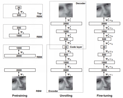
Fig. 1. Pretraining consists of learning a stack of restricted Boltzmann machines (RBMs), each having only one layer of feature detectors. The learned feature activations of one RBM are used as the ‘‘data’’ for training the next RBM in the stack. After the pretraining, the RBMs are ‘‘unrolled’’ to create a deep autoencoder, which is then fine-tuned using backpropagation of error derivatives.
- QUOTE: A simple and widely used method is principal components analysis (PCA), which finds the directions of greatest variance in the data set and represents each data point by its coordinates along each of these directions. We describe a nonlinear generalization of PCA that uses an adaptive, multilayer encoder network to transform the high-dimensional data into a low-dimensional code and a similar “decoder” network to recover the data from the code. Starting with random weights in the two networks, they can be trained together by minimizing the discrepancy between the original data and its reconstruction. The required gradients are easily obtained by using the chain rule to backpropagate error derivatives first through the decoder network and then through the encoder network (1). The whole system is called an “autoencoder” and is depicted in Fig. 1.
