Neural Network Backward Pass
A Neural Network Backward Pass is a Back-Propagation Algorithm that defines a Neural Network Hidden Layer that represents the state of backpropagation.
- AKA: Neural Network Backward State.
- Example(s):
- Counter-Example(s):
- See: Bidirectional Neural Network, ConvNet Network, RNN Network.
References
2018
- (Wikipedia, 2018) ⇒ https://www.wikiwand.com/en/Backpropagation#Pseudocode Retrieved: 2018-07-15.
- The following is pseudocode for a stochastic gradient descent algorithm for training a three-layer network (only one hidden layer):
do
forEach training example named ex
prediction = neural-net-output(network, ex) // forward pass
actual = teacher-output(ex)
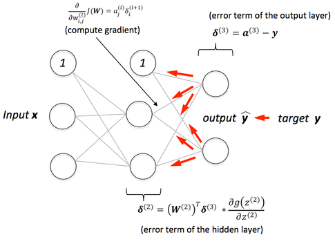
compute error (prediction - actual) at the output units
compute [math]\displaystyle{ \Delta w_h }[/math] for all weights from hidden layer to output layer // backward pass
compute [math]\displaystyle{ \Delta w_i }[/math] for all weights from input layer to hidden layer // backward pass continued update network weights // input layer not modified by error estimate
until all examples classified correctly or another stopping criterion satisfied
return the network
- The lines labeled "backward pass" can be implemented using the backpropagation algorithm, which calculates the gradient of the error of the network regarding the network's modifiable weights.[1]
2018c
- (Raven Protocol, 2018) ⇒ "Back-Propagation" In: https://medium.com/ravenprotocol/everything-you-need-to-know-about-neural-networks-6fcc7a15cb4 Retrieved: 2018-07-15
- QUOTE: After forward propagation we get an output value which is the predicted value. To calculate error we compare the predicted value with the actual output value. We use a loss function (mentioned below) to calculate the error value. Then we calculate the derivative of the error value with respect to each and every weight in the neural network. Back-Propagation uses chain rule of Differential Calculus. In chain rule first we calculate the derivatives of error value with respect to the weight values of the last layer. We call these derivatives, gradients and use these gradient values to calculate the gradients of the second last layer. We repeat this process until we get gradients for each and every weight in our neural network. Then we subtract this gradient value from the weight value to reduce the error value. In this way we move closer (descent) to the Local Minima(means minimum loss).
Backward Propagation
2016
- (wang, 2016) ⇒ Tingwu Wang (2016) Recurrent Neural Network Tutorial: http://www.cs.toronto.edu/~tingwuwang/rnn_tutorial.pdf
- QUOTE: 1. Algorithm looks like this:.
- QUOTE: 1. Algorithm looks like this:

2015
- (Urtasun & Zemel, 2015) ⇒ Raquel Urtasun, and Rich Zemel (2015). CSC 411: Lecture 10: Neural Networks I"
- QUOTE: We only need to know two algorithms:
- Forward pass: performs inference.
- Backward pass: performs learning
- QUOTE: We only need to know two algorithms:
2005
- (Graves & Schmidhuber, 2005) ⇒ Alex Graves and Jurgen Schmidhuber (2005). "Framewise phoneme classification with bidirectional LSTM and other neural network architectures" (PDF). Neural Networks, 18(5-6), 602-610. DOI 10.1016/j.neunet.2005.06.042
- QUOTE: Backward Pass
- Reset all partial derivatives to 0.
- Starting at time [math]\displaystyle{ \tau_1 }[/math], propagate the output errors backwards through the unfolded net, using the standard BPTT equations for a softmax output layer and the cross-entropy error function:
[math]\displaystyle{ define\; \delta_k(\tau)=\frac{\partial E(\tau)}{\partial x_k}; \quad \delta_k(\tau) = y_k(\tau ) − t_k(\tau)\quad k \in \text{output units} }[/math]
*** For each LSTM block the δ’s are calculated as follows:
Cell Outputs: [math]\displaystyle{ \forall c \in C,\; define\, \epsilon = \sum_{j\in N}w_{jc}\delta_j (\tau + 1) }[/math]
Output Gates: [math]\displaystyle{ \delta_w = f'(x_w)\sum_{c\in C}\epsilon_c h(s_c) }[/math]
States: [math]\displaystyle{ \frac{\partial E}{\partial s_c}(\tau)=\epsilon_c y_w h'(s_c)+\frac{\partial E}{\partial s_c}(\tau+1)y_\phi (\tau+1)+\delta_l(\tau + 1)w_{lc} + \delta_\phi(\tau + 1)w_{\phi c} + \delta _ww_{wc} }[/math]
Cells: [math]\displaystyle{ \forall c \in C, \delta_c = y_{l}g'(x_c)\frac{\partial E}{\partial s_c} }[/math]
Forget Gates:[math]\displaystyle{ \delta_\phi = f'(x_phi)\sum_{c\in C}\frac{\partial E}{\partial s_c} s_c(\tau -1) }[/math]
Input Gates: [math]\displaystyle{ \delta_l = f'(x_l)\sum_{c\in C}\frac{\partial E}{\partial s_c} g(x_c) }[/math]
- Using the standard BPTT equation, accumulate the δ’s to get the partial derivatives of the cumulative sequence error: [math]\displaystyle{ define\; E_{total}(S) = \sum^{\tau_1}_{\tau=\tau_0} E(\tau);\quad define\; \bigtriangledown_{ij} (S) = \frac{\partial E_{total}(S)}{\partial w_{ij}} \implies \bigtriangledown_{ij} (S)= \sum^{\tau_1}_{\tau=\tau_0+1} \delta_i(\tau)y_j (\tau − 1) }[/math]
- QUOTE: Backward Pass
1997
- (Schuster & Paliwal, 1997) ⇒ Mike Schuster, and Kuldip K. Paliwal. (1997). “Bidirectional Recurrent Neural Networks.” In: IEEE Transactions on Signal Processing Journal, 45(11). doi:10.1109/78.650093
- QUOTE: To overcome the limitations of a regular RNN outlined in the previous section, we propose a bidirectional recurrent neural network (BRNN) that can be trained using all available input information in the past and future of a specific time frame.
1) Structure: The idea is to split the state neurons of a regular RNN in a part that is responsible for the positive time direction (forward states) and a part for the negative time direction (backward states). Outputs from forward states are not connected to inputs of backward states, and vice versa. This leads to the general structure that can be seen in Fig. 3, where it is unfolded over three time steps.
.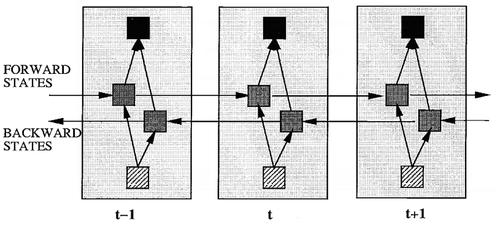
Fig. 3. General structure of the bidirectional recurrent neural network (BRNN) shown unfolded in time for three time steps
(...) The training procedure for the unfolded bidirectional network over time can be summarized as follows.
- QUOTE: To overcome the limitations of a regular RNN outlined in the previous section, we propose a bidirectional recurrent neural network (BRNN) that can be trained using all available input information in the past and future of a specific time frame.

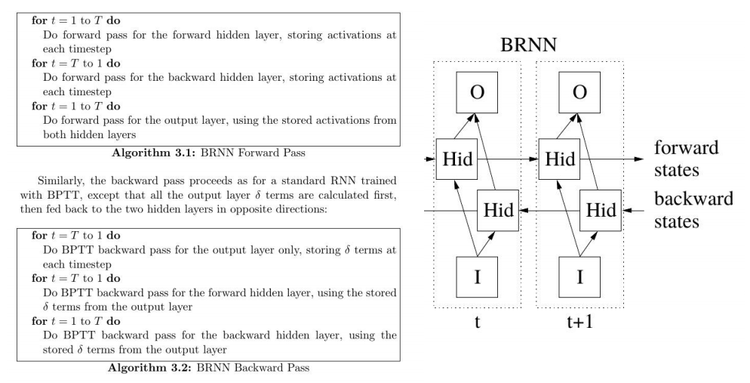
- 1) FORWARD PASS
- Run all input data for one time slice [math]\displaystyle{ 1 \lt t \leq T }[/math]through the BRNN and determine all predicted outputs.
- a) Do forward pass just for forward states (from [math]\displaystyle{ t=1 }[/math] to [math]\displaystyle{ t=T }[/math]) and backward states (from [math]\displaystyle{ t=T }[/math] to [math]\displaystyle{ t=1 }[/math]).
- b) Do forward pass for output neurons.
- 2) BACKWARD PASS
- Calculate the part of the objective function derivative for the time slice [math]\displaystyle{ 1 \lt t \leq T }[/math] used in the forward pass.
- a) Do backward pass for output neurons.
- b) Do backward pass just for forward states (from [math]\displaystyle{ t=T }[/math] to [math]\displaystyle{ t=1 }[/math]) and backward states (from [math]\displaystyle{ t=1 }[/math] to [math]\displaystyle{ t=T }[/math]).
- 3) UPDATE WEIGHTS