3-Layer ANN Training System
A 3-Layer ANN Training System is an n-layer ANN training system that implements a 3-Layer ANN Training Algorithm to solve a 3-Layer ANN training task (which requires a 3-layer ANN).
- AKA: Two Hidden-Layer ANN Training System.
- Context:
- It is based on a 3-Layer ANN Mathematical Model.
- Example(s):
- A 3-Layer Feed-Forward Neural Network Training System applied to Sigmoid Neurons such as:
- (Trask, 2015) ⇒ https://github.com/pkumusic/10701_Coding/blob/master/Neural%20Network/3-nn.py
- (CS231n, 2018) ⇒ Example feed-forward computation
- a 3-Layer Google's Tensorflow Neural Network Training System
- A 3-Layer Feed-Forward Neural Network Training System applied to Sigmoid Neurons such as:
- Counter-Examples:
- See: N-Layer Neural Network, Artificial Neural Network, Neural Network Layer, Artificial Neuron, Neuron Activation Function, Neural Network Topology.
References
2018
- (CS231n, 2018) ⇒ Example feed-forward computation. In: CS231n Convolutional Neural Networks for Visual Recognition Retrieved: 2018-01-14.
- QUOTE: Repeated matrix multiplications interwoven with activation function. One of the primary reasons that Neural Networks are organized into layers is that this structure makes it very simple and efficient to evaluate Neural Networks using matrix vector operations. Working with the example three-layer neural network in the diagram above, the input would be a [3x1] vector. All connection strengths for a layer can be stored in a single matrix. For example, the first hidden layer’s weights
W1would be of size [4x3], and the biases for all units would be in the vectorb1, of size [4x1]. Here, every single neuron has its weights in a row ofW1, so the matrix vector multiplicationnp.dot(W1,x)evaluates the activations of all neurons in that layer. Similarly,W2would be a [4x4] matrix that stores the connections of the second hidden layer, andW3a [1x4] matrix for the last (output) layer. The full forward pass of this 3-layer neural network is then simply three matrix multiplications, interwoven with the application of the activation function:
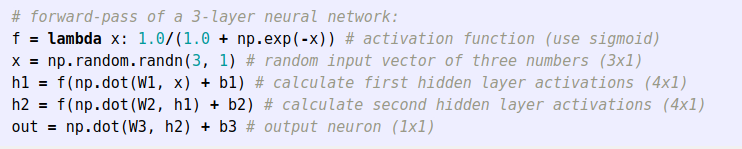
In the above code,
W1,W2,W3,b1,b2,b3are the learnable parameters of the network. Notice also that instead of having a single input column vector, the variablexcould hold an entire batch of training data (where each input example would be a column ofx) and then all examples would be efficiently evaluated in parallel. Notice that the final Neural Network layer usually doesn’t have an activation function (e.g. it represents a (real-valued) class score in a classification setting).The forward pass of a fully-connected layer corresponds to one matrix multiplication followed by a bias offset and an activation function.
- QUOTE: Repeated matrix multiplications interwoven with activation function. One of the primary reasons that Neural Networks are organized into layers is that this structure makes it very simple and efficient to evaluate Neural Networks using matrix vector operations. Working with the example three-layer neural network in the diagram above, the input would be a [3x1] vector. All connection strengths for a layer can be stored in a single matrix. For example, the first hidden layer’s weights

2015
- (Trask, 2015) ⇒ Trask (July 15, 2015). “Part 2: A Slightly Harder Problem". In: A Neural Network in 11 lines of Python (Part 1)
- QUOTE: In order to first combine pixels into something that can then have a one-to-one relationship with the output, we need to add another layer. Our first layer will combine the inputs, and our second layer will then map them to the output using the output of the first layer as input. Before we jump into an implementation though, take a look at this table.
| Inputs (l0) | Hidden Weights (l1) | Output (l2) | |||||
| 0 | 0 | 1 | 0.1 | 0.2 | 0.5 | 0.2 | 0 |
| 0 | 1 | 1 | 0.2 | 0.6 | 0.7 | 0.1 | 1 |
| 1 | 0 | 1 | 0.3 | 0.2 | 0.3 | 0.9 | 1 |
| 1 | 1 | 1 | 0.2 | 0.1 | 0.3 | 0.8 | 0 |
- If we randomly initialize our weights, we will get hidden state values for layer 1. Notice anything? The second column (second hidden node), has a slight correlation with the output already! It's not perfect, but it's there. Believe it or not, this is a huge part of how neural networks train. (Arguably, it's the only way that neural networks train.) What the training below is going to do is amplify that correlation. It's both going to update syn1 to map it to the output, and update syn0 to be better at producing it from the input!
- Note: The field of adding more layers to model more combinations of relationships such as this is known as "deep learning" because of the increasingly deep layers being modeled (...)