Gradient-Descent Boosted Training (GBM) Algorithm
A Gradient-Descent Boosted Training (GBM) Algorithm is an boosted ensemble learning algorithm that is a gradient-descent algorithm which employs gradient descent optimization to build models sequentially in a way that each new model incrementally reduces the residual errors of the previous models.
- Context:
- It can (typically) operate by sequentially adding predictors to an ensemble, each one correcting its predecessor.
- It can be used for both classification and regression tasks.
- It can handle various data types, including categorical and continuous variables.
- It can be sensitive to overfitting if the number of trees is too large or the learning rate is too high.
- It can be computationally demanding, requiring careful tuning of parameters and adequate computing resources.
- It can be implemented by a Gradient Descent Boosted Training System (to solve a gradient descent boosted training task).
- It can range from being a Gradient Boosting Estimation Algorithm to being a Gradient Boosting Ranking Algorithm to being a Gradient Boosting Classification Algorithm.
- It can be solved by a Gradient-Descent Boosted Training System (to solve a gradient boosting task).
- It can identify shortcomings in previous model via Negative Gradients (aka pseudo residuals).
- ...
- Example(s):
- Counter-Example(s):
- See: Boosting Algorithm, Decision Tree Training Algorithm, Gradient Descent Algorithm, Iterative Gradient Descent Algorithm; Ensemble Learning, Boosting Meta-Algorithm, Differentiable Function.
References
2024
- (Wikipedia, 2024) ⇒ https://en.wikipedia.org/wiki/Gradient_boosting Retrieved:2024-3-13.
- Gradient boosting is a machine learning technique based on boosting in a functional space, where the target is pseudo-residuals rather than the typical residuals used in traditional boosting. It gives a prediction model in the form of an ensemble of weak prediction models, i.e., models that make very few assumptions about the data, which are typically simple decision trees. [1] When a decision tree is the weak learner, the resulting algorithm is called gradient-boosted trees; it usually outperforms random forest.[2][1] A gradient-boosted trees model is built in a stage-wise fashion as in other boosting methods, but it generalizes the other methods by allowing optimization of an arbitrary differentiable loss function.
2015
- (Wikipedia, 2015) ⇒ http://en.wikipedia.org/wiki/Gradient_boosting Retrieved:2015-6-24.
- Gradient boosting is a machine learning technique for regression and classification problems, which produces a prediction model in the form of an ensemble of weak prediction models, typically decision trees. It builds the model in a stage-wise fashion like other boosting methods do, and it generalizes them by allowing optimization of an arbitrary differentiable loss function.
The idea of gradient boosting originated in the observation by Leo Breiman [3] that boosting can be interpreted as an optimization algorithm on a suitable cost function. Explicit regression gradient boosting algorithms were subsequently developed by Jerome H. Friedman[4] [5] simultaneously with the more general functional gradient boosting perspective of Llew Mason, Jonathan Baxter, Peter Bartlett and Marcus Frean
The latter two papers introduced the abstract view of boosting algorithms as iterative functional gradient descent algorithms. That is, algorithms that optimize a cost functional over function space by iteratively choosing a function (weak hypothesis) that points in the negative gradient direction. This functional gradient view of boosting has led to the development of boosting algorithms in many areas of machine learning and statistics beyond regression and classification.
- Gradient boosting is a machine learning technique for regression and classification problems, which produces a prediction model in the form of an ensemble of weak prediction models, typically decision trees. It builds the model in a stage-wise fashion like other boosting methods do, and it generalizes them by allowing optimization of an arbitrary differentiable loss function.
2017
- (Wikipedia, 2017) ⇒ https://en.wikipedia.org/wiki/Gradient_boosting#Algorithm Retrieved:2017-1-21.
- … Gradient boosting method assumes a real-valued y and seeks an approximation [math]\displaystyle{ \hat{F}(x) }[/math] in the form of a weighted sum of functions [math]\displaystyle{ h_i (x) }[/math] from some class ℋ, called base (or weak) learners: : [math]\displaystyle{ F(x) = \sum_{i=1}^M \gamma_i h_i(x) + \mbox{const} }[/math] .
In accordance with the empirical risk minimization principle, the method tries to find an approximation [math]\displaystyle{ \hat{F}(x) }[/math] that minimizes the average value of the loss function on the training set. It does so by starting with a model, consisting of a constant function [math]\displaystyle{ F_0(x) }[/math] , and incrementally expanding it in a greedy fashion: : [math]\displaystyle{ F_0(x) = \underset{\gamma}{\arg\min} \sum_{i=1}^n L(y_i, \gamma) }[/math] , : [math]\displaystyle{ F_m(x) = F_{m-1}(x) + \underset{f \in \mathcal{H}}{\operatorname{arg\,min}} \sum_{i=1}^n L(y_i, F_{m-1}(x_i) + f(x_i)) }[/math] ,
where is restricted to be a function from the class ℋ of base learner functions.
However, the problem of choosing at each step the best for an arbitrary loss function is a hard optimization problem in general, and so we'll "cheat" by solving a much easier problem instead.
The idea is to apply a steepest descent step to this minimization problem. If we only cared about predictions at the points of the training set, and were unrestricted, we'd update the model per the following equation, where we view [math]\displaystyle{ L(y, f) }[/math] not as a function of , but as a function of a vector of values [math]\displaystyle{ f(x_1), \ldots, f(x_n) }[/math] : : [math]\displaystyle{ F_m(x) = F_{m-1}(x) - \gamma_m \sum_{i=1}^n \nabla_{F_{m-1}} L(y_i, F_{m-1}(x_i)), }[/math] : [math]\displaystyle{ \gamma_m = \underset{\gamma}{\arg\min} \sum_{i=1}^n L\left(y_i, F_{m-1}(x_i) - \gamma \frac{\partial L(y_i, F_{m-1}(x_i))}{\partial F_{m-1}(x_i)} \right). }[/math] But as must come from a restricted class of functions (that's what allows us to generalize), we'll just choose the one that most closely approximates the gradient of . Having chosen, the multiplier is then selected using line search just as shown in the second equation above.
In pseudocode, the generic gradient boosting method is:
Input: training set [math]\displaystyle{ \{(x_i, y_i)\}_{i=1}^n, }[/math] a differentiable loss function [math]\displaystyle{ L(y, F(x)), }[/math] number of iterations .
Algorithm:
- Initialize model with a constant value:
- [math]\displaystyle{ F_0(x) = \underset{\gamma}{\arg\min} \sum_{i=1}^n L(y_i, \gamma). }[/math] # For = 1 to :
- Compute so-called pseudo-residuals:
- [math]\displaystyle{ r_{im} = -\left[\frac{\partial L(y_i, F(x_i))}{\partial F(x_i)}\right]_{F(x)=F_{m-1}(x)} \quad \mbox{for } i=1,\ldots,n. }[/math] ## Fit a base learner [math]\displaystyle{ h_m(x) }[/math] to pseudo-residuals, i.e. train it using the training set [math]\displaystyle{ \{(x_i, r_{im})\}_{i=1}^n }[/math] .
- Compute multiplier [math]\displaystyle{ \gamma_m }[/math] by solving the following one-dimensional optimization problem:
- [math]\displaystyle{ \gamma_m = \underset{\gamma}{\operatorname{arg\,min}} \sum_{i=1}^n L\left(y_i, F_{m-1}(x_i) + \gamma h_m(x_i)\right). }[/math] ## Update the model:
- [math]\displaystyle{ F_m(x) = F_{m-1}(x) + \gamma_m h_m(x). }[/math] # Output [math]\displaystyle{ F_M(x). }[/math]
- Initialize model with a constant value:
- … Gradient boosting method assumes a real-valued y and seeks an approximation [math]\displaystyle{ \hat{F}(x) }[/math] in the form of a weighted sum of functions [math]\displaystyle{ h_i (x) }[/math] from some class ℋ, called base (or weak) learners: : [math]\displaystyle{ F(x) = \sum_{i=1}^M \gamma_i h_i(x) + \mbox{const} }[/math] .
2016
- http://arogozhnikov.github.io/2016/06/24/gradient_boosting_explained.html
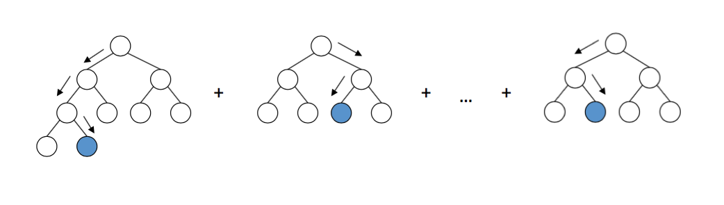
- QUOTE: Gradient boosting builds an ensemble of trees one-by-one, then the predictions of the individual trees are summed: [math]\displaystyle{ D(x)= d_\text{tree 1}(x)+d_\text{tree 2}(x)+... D(\mathbf{x}) = d_\text{tree 1}(\mathbf{x}) + d_\text{tree 2}(\mathbf{x}) + … D(x)=d_\text{tree 1}(x)+d_\text{tree 2}(x)+... }[/math] The next decision tree tries to cover the discrepancy between the target function [math]\displaystyle{ f(x) f(\mathbf{x}) f(x) }[/math] and the current ensemble prediction by reconstructing the residual.
For example, if an ensemble has 3 trees the prediction of that ensemble is: D(x)=dtree 1(x)+dtree 2(x)+dtree 3(x) D(\mathbf{x}) = d_\text{tree 1}(\mathbf{x}) + d_\text{tree 2}(\mathbf{x}) + d_\text{tree 3}(\mathbf{x}) D(x)=dtree 1(x)+dtree 2(x)+dtree 3(x) The next tree (tree 4 \text{tree 4} tree 4 ) in the ensemble should complement well the existing trees and minimize the training error of the ensemble.
In the ideal case we'd be happy to have: [math]\displaystyle{ D(x)+d_\text{tree 4}(x)=f(x). D(\mathbf{x}) + d_\text{tree 4}(\mathbf{x}) = f(\mathbf{x}). D(x)+dtree 4(x)=f(x) }[/math].
To get a bit closer to the destination, we train a tree to reconstruct the difference between the target function and the current predictions of an ensemble, which is called the residual: R(x)=f(x)−D(x). R(\mathbf{x}) = f(\mathbf{x}) - D(\mathbf{x}). R(x)=f(x)−D(x). Did you notice? If decision tree completely reconstructs R(x) R(\mathbf{x}) R(x), the whole ensemble gives predictions without errors (after adding the newly-trained tree to the ensemble)! That said, in practice this never happens, so we instead continue the iterative process of ensemble building.
- QUOTE: Gradient boosting builds an ensemble of trees one-by-one, then the predictions of the individual trees are summed: [math]\displaystyle{ D(x)= d_\text{tree 1}(x)+d_\text{tree 2}(x)+... D(\mathbf{x}) = d_\text{tree 1}(\mathbf{x}) + d_\text{tree 2}(\mathbf{x}) + … D(x)=d_\text{tree 1}(x)+d_\text{tree 2}(x)+... }[/math] The next decision tree tries to cover the discrepancy between the target function [math]\displaystyle{ f(x) f(\mathbf{x}) f(x) }[/math] and the current ensemble prediction by reconstructing the residual.
2015
- http://slideshare.net/DeepakGeorge5/decision-tree-ensembles-bagging-random-forest-gradient-boosting-machines/15
- QUOTE:
- AdaBoost is equivalent to forward stagewise additive modeling using the exponential loss function.
- Generalization of AdaBoost to work with arbitrary loss functions resulted in GBM. Gradient Boosting = Gradient Descent + Boosting
- GBM uses gradient descent algorithm which can optimize any differentiable loss function.
- In Adaboost, ‘shortcomings’ are identified by high-weight data points.
- In Gradient Boosting, “shortcomings” are identified by negative gradients (also called pseudo residuals).
- In GBM instead of reweighting used in adaboost, each new tree is fit to the negative gradients of the previous tree.
- Each tree in GBM is a successive gradient descent step.
- QUOTE:
2012
- (Natarajan et al., 2012) ⇒ Sriraam Natarajan, Tushar Khot, Kristian Kersting, Bernd Gutmann, and Jude Shavlik. (2012). “Gradient-based Boosting for Statistical Relational Learning: The Relational Dependency Network Case.” In: Machine Learning, 86(1).
2010
- (Seni & Elder, 2010) ⇒ Giovanni Seni, and John F. Elder. (2010). “Ensemble Methods in Data Mining: Improving Accuracy Through Combining Predictions.” Morgan & Claypool. doi:10.2200/S00240ED1V01Y200912DMK002
- QUOTE: The ISLE framework allows us to view the classic ensemble methods of Bagging, Random Forest, AdaBoost, and Gradient Boosting as special cases of a single algorithm.
2002
- (Friedman, 2002) ⇒ Jerome H. Friedman. (2002). “Stochastic Gradient Boosting.” In: Computational Statistics & Data Analysis 38, no. 4
2001
- (Friedman, 2001) ⇒ Jerome H. Friedman. (2001). “Greedy Function Approximation: A gradient boosting machine.” In: The Annals of Statistics, 29(5) doi:10.1214/aos/1013203451
- QUOTE: Function estimation/approximation is viewed from the perspective of numerical optimization in function space, rather than parameter space. A connection is made between stagewise additive expansions and steepest-descent minimization. A general gradient descent "boosting" paradigm is developed for additive expansions based on any fitting criterion.
- ↑ 1.0 1.1 Cite error: Invalid
<ref>tag; no text was provided for refs namedhastie - ↑ Cite error: Invalid
<ref>tag; no text was provided for refs named:1 - ↑ Brieman, L. “Arcing The Edge" (June 1997)
- ↑ Friedman, J. H. “Greedy Function Approximation: A Gradient Boosting Machine." (February 1999)
- ↑ Friedman, J. H. “Stochastic Gradient Boosting." (March 1999)
- ↑
- ↑