Attention Mechanism
A Attention Mechanism is a neural network component within a memory augmented neural network that allows the model to dynamically focus on certain parts of its input or its own internal state (memory) that are most relevant for performing a given task.
- AKA: Neural Attention Model, Neural Network Attention System.
- Context:
- It can typically be incorporated into a Neural Network with Attention Mechanism to enable dynamic focusing on relevant information during processing.
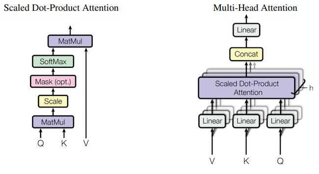
- It can typically utilize an Attention Pattern Matrix that encodes the pairwise relevance between attention input tokens, allowing the model to selectively focus on different parts of the input when updating each token's representation.
- It can typically compute Attention Scores between attention query vectors (representing the current state) and attention key vectors (representing the input elements), which are then normalized using an attention softmax function to obtain attention weights.
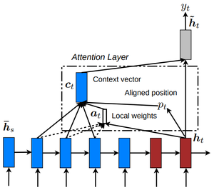
- It can typically use the computed Attention Weights to take a weighted sum of attention value vectors, which correspond to the input elements, to obtain an attention context vector that captures the most relevant information for the current state.
- It can typically update its Attention Query Vectors, Attention Key Vectors, and Attention Value Vectors through learnable linear transformations, allowing the model to adapt and learn the most suitable representations for the given task during training.
- It can be defined by an Attention Function, which mathematically determines how attention scores are computed between input elements.
- It can range from being a Local Attention Mechanism to being a Global Attention Mechanism, depending on its attention scope.
- It can range from being a Self-Attention Mechanism to being a Cross-Attention Mechanism, depending on its attention source-target relationship.
- It can range from being an Additive Attention Mechanism to being a Multiplicative Attention Mechanism, depending on its attention scoring method.
- It can range from being a Deterministic Attention Mechanism to being a Stochastic Attention Mechanism, depending on its attention weight determination approach.
- It can range from being a Soft Attention Mechanism to being a Hard Attention Mechanism, depending on its attention weight distribution characteristic.
- It can range from being a Single-Head Attention Mechanism to being a Multi-Head Attention Mechanism, depending on its attention processing parallelism.
- It can significantly improve Neural Network Performance on tasks requiring selective information processing such as attention-based machine translation, attention-based document summarization, and attention-based image captioning.
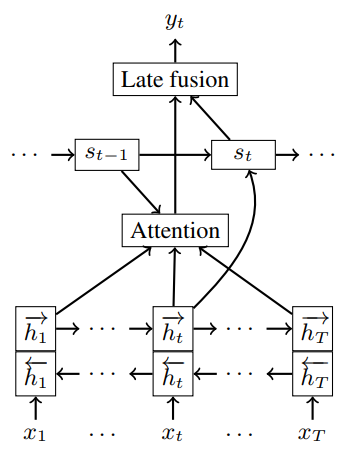
- It can alleviate the Information Bottleneck Problem in encoder-decoder architectures by allowing the decoder to access all encoder states rather than just a fixed-length context vector.
- It can be analyzed through Attention Mechanism Computational Complexity Analysis to optimize implementation efficiency.
- ...
- Examples:
- Attention Mechanism Classifications by scoring method, such as:
- Content-Based Attention Mechanisms, such as:
- Additive Attention Mechanism, computing attention weights by using a feed-forward network with a single hidden layer to combine query and key vectors, enabling complex non-linear relationships.
- Multiplicative Attention Mechanisms, such as:
- Scaled Dot-Product Attention Mechanism, scaling dot products by the dimensionality of the vectors to improve stability in models with large dimension sizes.
- Cosine Similarity Attention Mechanism, using normalized vectors to compute attention scores for length-invariant matching.
- Content-Based Attention Mechanisms, such as:
- Attention Mechanism Classifications by attention scope, such as:
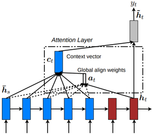
- Global Attention Mechanism, attending to all source positions to generate a context vector through weighted averaging of all source states.
- Local Attention Mechanism, focusing on a subset of source positions through a predicted alignment position and an attention window, reducing computational complexity.
- Attention Mechanism Applications by task domain, such as:
- Natural Language Processing Attention Mechanisms, such as:
- Encoder-Decoder Attention Mechanism, widely used in sequence-to-sequence models for tasks such as machine translation, allowing the decoder to attend over all positions in the input sequence.
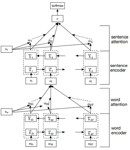
- Hierarchical Attention Mechanism, employing multiple levels of attention such as word-level and sentence-level attention for document classification.
- Computer Vision Attention Mechanisms, such as:
- Visual Attention Mechanism, selectively focusing on parts of an image for tasks like image captioning and visual question answering.
- Natural Language Processing Attention Mechanisms, such as:
- Attention Mechanism Variants by design characteristics, such as:
- Multi-Head Attention Mechanism, running several attention mechanisms in parallel to capture different types of relationships in the input data.
- Hard Stochastic Attention Mechanism, where attention decisions are sampled from a probability distribution, leading to discrete attention focusing.
- Block Sparse Attention Mechanism, introducing sparsity by computing attention within blocks or between specific blocks, reducing computational complexity.
- Grouped Query Attention Mechanism, effectively combining elements of Multi-Head Attention Mechanism and Multi-Query Attention Mechanism for improved efficiency.
- ...
- Attention Mechanism Classifications by scoring method, such as:
- Counter-Examples:
- Self-Attention Mechanism without Positional Encoding, which lacks the ability to incorporate positional information that standard attention mechanisms provide, limiting its effectiveness for sequential or spatial data.
- Uniform Attention Distribution, which assigns equal weight to all input elements rather than selectively focusing as attention mechanisms do, reducing effectiveness for tasks requiring selective processing.
- Static Attention Mechanism, where attention weights are fixed rather than dynamically computed as in proper attention mechanisms, limiting adaptability to different inputs.
- Gating Mechanism such as in Gated Recurrent Unit, which controls information flow but lacks the fine-grained selective focusing capability of attention mechanisms.
- Sequential Memory Cell such as in Long Short-Term Memory Unit, which retains information over time but doesn't implement dynamic importance weighting across input elements that attention mechanisms provide.
- Convolutional Neural Network Layer, which applies fixed spatial filters rather than computing dynamic attention patterns based on content relevance.
- See: Transformer Model, Sequence-to-Sequence Model with Attention, Attention Alignment, Attention Layer, Attention Map, Attention Weight Distribution, Neural Memory Architecture, Attentional Neural Network.
References
2018a
- (Brown et al., 2018) ⇒ Andy Brown, Aaron Tuor, Brian Hutchinson, and Nicole Nichols. (2018). “Recurrent Neural Network Attention Mechanisms for Interpretable System Log Anomaly Detection.” In: Proceedings of the First Workshop on Machine Learning for Computing Systems (MLCS'18). ISBN:978-1-4503-5865-1 doi:10.1145/3217871.3217872
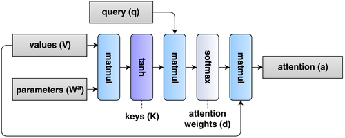
- QUOTE: In this work we use dot product attention (Figure 3), wherein an “attention vector” a is generated from three values: 1) a key matrix $\mathbf{K}$, 2) a value matrix \mathbf{V}, and 3) a query vector \mathbf{q}. In this formulation, keys are a function of the value matrix:
- QUOTE: In this work we use dot product attention (Figure 3), wherein an “attention vector” a is generated from three values: 1) a key matrix $\mathbf{K}$, 2) a value matrix \mathbf{V}, and 3) a query vector \mathbf{q}. In this formulation, keys are a function of the value matrix:
| [math]\displaystyle{ \mathbf{K} = \tanh\left(\mathbf{VW}^a\right) }[/math] | (5) |
- parameterized by $\mathbf{W}a$ . The importance of each timestep is determined by the magnitude of the dot product of each key vector with the query vector $\mathbf{q} \in \R^{La}$ for some attention dimension hyperparameter, $La$. These magnitudes determine the weights, $\mathbf{d}$ on the weighted sum of value vectors, $\mathbf{a}$:
- parameterized by $\mathbf{W}a$ . The importance of each timestep is determined by the magnitude of the dot product of each key vector with the query vector $\mathbf{q} \in \R^{La}$ for some attention dimension hyperparameter, $La$. These magnitudes determine the weights, $\mathbf{d}$ on the weighted sum of value vectors, $\mathbf{a}$:
| [math]\displaystyle{ \begin{align} \mathbf{d} &= \mathrm{softmax}\left(\mathbf{qKT} \right) \\ \mathbf{a} &= \mathbf{dV} \end{align} }[/math] | (6) |
| (7) |
|
2018b
- (Yogatama et al., 2018) ⇒ Dani Yogatama, Yishu Miao, Gabor Melis, Wang Ling, Adhiguna Kuncoro, Chris Dyer, and Phil Blunsom. (2018). “Memory Architectures in Recurrent Neural Network Language Models.” In: Proceedings of 6th International Conference on Learning Representations.
- QUOTE: Random access memory. One common approach to retrieve information from the distant past more reliably is to augment the model with a random access memory block via an attention based method. In this model, we consider the previous $K$ states as the memory block, and construct a memory vector $\mathbf{m}_t$ by a weighted combination of these states:[math]\displaystyle{ \mathbf{m}_t = \displaystyle \sum_{i=t−K}^{t−1} a_i\mathbf{h}_i \quad }[/math], where [math]\displaystyle{ \quad a_i \propto \exp\left(\mathbf{w}_{m,i}\mathbf{h}_i + \mathbf{w}_{m,h} \mathbf{h}_t\right) }[/math]
- QUOTE: Random access memory. One common approach to retrieve information from the distant past more reliably is to augment the model with a random access memory block via an attention based method. In this model, we consider the previous $K$ states as the memory block, and construct a memory vector $\mathbf{m}_t$ by a weighted combination of these states:
2017a
- (Gupta et al., 2017) ⇒ Rahul Gupta, Soham Pal, Aditya Kanade, and Shirish Shevade. (2017). “DeepFix: Fixing Common C Language Errors by Deep Learning.” In: Proceeding of AAAI.
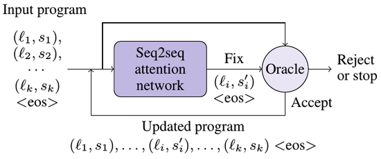
- QUOTE: We present an end-to-end solution, called DeepFix, that does not use any external tool to localize or fix errors. We use a compiler only to validate the fixes suggested by DeepFix. At the heart of DeepFix is a multi-layered sequence-to-sequence neural network with attention (Bahdanau, Cho, and Bengio 2014), comprising of an encoder recurrent neural network (RNN) to process the input and a decoder RNN with attention that generates the output. The network is trained to predict an erroneous program location along with the correct statement. DeepFix invokes it iteratively to fix multiple errors in the program one-by-one. (...)
DeepFix uses a simple yet effective iterative strategy to fix multiple errors in a program as shown in Figure 2 (...)
- QUOTE: We present an end-to-end solution, called DeepFix, that does not use any external tool to localize or fix errors. We use a compiler only to validate the fixes suggested by DeepFix. At the heart of DeepFix is a multi-layered sequence-to-sequence neural network with attention (Bahdanau, Cho, and Bengio 2014), comprising of an encoder recurrent neural network (RNN) to process the input and a decoder RNN with attention that generates the output. The network is trained to predict an erroneous program location along with the correct statement. DeepFix invokes it iteratively to fix multiple errors in the program one-by-one. (...)
|
2017b
- (See et al., 2017) ⇒ Abigail See, Peter J. Liu, and Christopher D. Manning. (2017). “Get To The Point: Summarization with Pointer-Generator Networks.” In: Proceedings of the 55th Annual Meeting of the Association for Computational Linguistics (Volume 1: Long Papers). DOI:10.18653/v1/P17-1099.
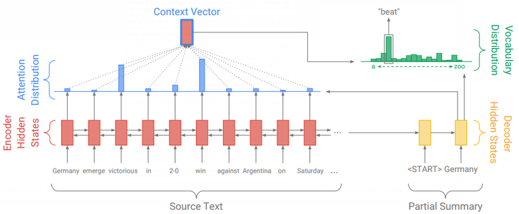
- QUOTE: The attention distribution at is calculated as in Bahdanau et al. (2015):
| [math]\displaystyle{ \begin{align} e^t_i &= \nu^T \mathrm{tanh}\left(W_hh_i +W_sS_t +b_{attn}\right) \\ a^t &= \mathrm{softmax}\left(e^t \right) \end{align} }[/math] | (1) |
| (2) |
- where $\nu$, $W_h$, $W_s$ and $b_{attn}$ are learnable parameters. The attention distribution can be viewed as a probability distribution over the source words, that tells the decoder where to look to produce the next word. Next, the attention distribution is used to produce a weighted sum of the encoder hidden states, known as the context vector $h^*_t$
- where $\nu$, $W_h$, $W_s$ and $b_{attn}$ are learnable parameters. The attention distribution can be viewed as a probability distribution over the source words, that tells the decoder where to look to produce the next word. Next, the attention distribution is used to produce a weighted sum of the encoder hidden states, known as the context vector $h^*_t$
| [math]\displaystyle{ h^∗_t = \displaystyle\sum_i a^t_i h_i }[/math] | (3) |
|
2017c
- (Synced Review, 2017) ⇒ Synced (2017). “A Brief Overview of Attention Mechanism.” In: Medium - Synced Review Blog Post.
- QUOTE: And to build context vector is fairly simple. For a fixed target word, first, we loop over all encoders' states to compare target and source states to generate scores for each state in encoders. Then we could use softmax to normalize all scores, which generates the probability distribution conditioned on target states. At last, the weights are introduced to make context vector easy to train. That’s it. Math is shown below:
| [math]\displaystyle{ \begin{align} \alpha_{ts} &=\dfrac{\exp\left(\mathrm{score}\left(\mathbf{h}_t,\mathbf{\overline{h}}_s\right)\right)}{\displaystyle\sum_{s'=1}^S \exp\left(\mathrm{score}\left(\mathbf{h}_t,\mathbf{\overline{h}}_{s'}\right)\right)}\\ \mathbf{c}_t &=\displaystyle\sum_s \alpha_{ts}\mathbf{\overline{h}}_s\\ \mathbf{a}_t &=f\left(\mathbf{c}_t,\mathbf{h}_t\right) = \mathrm{tanh}\left(\mathbf{W}_c\big[\mathbf{c}_t; \mathbf{h}_t\big]\right) \end{align} }[/math] | [Attention weights] | (1) |
| [Context vector] | (2) | |
| [Attention vector] | (3) |
- To understand the seemingly complicated math, we need to keep three key points in mind:
- 1. During decoding, context vectors are computed for every output word. So we will have a 2D matrix whose size is # of target words multiplied by # of source words. Equation (1) demonstrates how to compute a single value given one target word and a set of source word.
- 2. Once context vector is computed, attention vector could be computed by context vector, target word, and attention function $f$.
- 3. We need attention mechanism to be trainable. According to [equation (4), both styles offer the trainable weights (W in Luong’s, W1 and W2 in Bahdanau’s). Thus, different styles may result in different performance.
- To understand the seemingly complicated math, we need to keep three key points in mind:
2016a
2016c
2015a
(...)
2015b
2015b
2015c
2015d
|
