1999 InductiveLearningofTreebasedReg
- (Torgo, 1999) ⇒ Luis Torgo. (1999). “Inductive Learning of Tree-based Regression Models.” Ph.D. Thesis, Thesis, Faculty of Sciences, University of Porto
Subject Headings: Regression Tree Induction, Regression Tree Induction Algorithm.
Notes
Cited By
Quotes
Abstract
This thesis explores different aspects of the induction of tree-based regression models from data. The main goal of this study is to improve the predictive accuracy of regression trees, while retaining as much as possible their comprehensibility and computational efficiency. Our study is divided in three main parts.
In the first part we describe in detail two different methods of growing a regression tree: minimising the mean squared error and minimising the mean absolute deviation. Our study is particularly focussed on the computational efficiency of these tasks. We present several new algorithms that lead to significant computational speed-ups. We also describe an experimental comparison of both methods of growing a regression tree highlighting their different application goals.
Pruning is a standard procedure within tree-based models whose goal is to provide a good compromise for achieving simple and comprehensible models with good predictive accuracy. In the second part of our study we describe a series of new techniques for pruning by selection from a series of alternative pruned trees. We carry out an extensive set of experiments comparing different methods of pruning, which show that our proposed techniques are able to significantly outperform the predictive accuracy of current state of the art pruning algorithms in a large set of regression domains.
In the final part of our study we present a new type of tree-based models that we refer to as local regression trees. These hybrid models integrate tree-based regression with local modelling techniques. We describe different types of local regression trees and show that these models are able to significantly outperform standard regression trees in terms of predictive accuracy. Through a large set of experiments we prove the competitiveness of local regression trees when compared to existing regression techniques.
Chapter 1. Introduction
Chapter 2. Inductive Learning
Chapter 3. Tree-based Regression
This chapter describes two different approaches to induce regression trees. We first present the standard methodology based on the minimisation of the squared error. Least squares (LS) regression trees had already been described in detail in the book by Breiman et. al. (1984). Compared to this work we present some simplifications of the splitting criterion that lead to gains in computational efficiency. We then address the alternative method of using a least absolute deviation (LAD) error criterion to obtain regression trees. Although mentioned in the book of Breiman and colleagues (1984), this methodology was never described in sufficient detail. In this chapter we present such a description. The LAD criterion is known to be more robust to skewed distributions and outliers than the LS criterion used in standard regression trees. However, the use of the LAD criterion brings additional computational difficulties to the task of growing a tree. In this chapter we present algorithms based on a theoretical study of the LAD criterion that overcome these difficulties for numeric variables. With respect to nominal variables we show that the theorem proved by Breiman et. al. (1984) for subset splits in LS trees does not hold for the LAD error criterion. Still, we have experimentally observed that the use of the results of this theorem as a heuristic method of obtaining the best split does not degrade predictive accuracy. Moreover, using this heuristic brings significant gains in computation efficiency.
…
3.1 Tree-based Models
Work on tree-based regression models traces back to Morgan and Sonquist (1963) and their AID program. However, the major reference on this research line still continuous to be the seminal book on classification and regression trees by Breiman and his colleagues (1984). These authors provide a thorough description of both classification and regression tree-based models. Within Machine Learning, most research efforts concentrate on classification (or decision) trees (Hunt et al.,1966; Quinlan, 1979; Kononenko et al.,1984).
Work on regression trees started with RETIS (Karalic & Cestnik, 1991) and M5 (Quinlan, 1992). Compared to CART (Breiman et. al.,1984), RETIS uses a different pruning methodology based on the Niblet and Bratko (1986) algorithm and m-estimates (Cestnik, 1990). With respect to M5 (Quinlan, 1992), its novelty results from the use of linear regression models in the tree leaves19. A further extension of M5 was described in Quinlan (1993). This extension consisted in combining the predictions of the trees with k nearest neighbour models.
Tree-based regression models are known for their simplicity and efficiency when dealing with domains with large number of variables and cases. Regression trees are obtained using a fast divide and conquer greedy algorithm that recursively partitions the given training data into smaller subsets. The use of this algorithm is the cause of the efficiency of these methods. However, it can also lead to poor decisions in lower levels of the tree due to the unreliability of estimates based on small samples of cases. Methods to deal with this problem turn out to be nearly as important as growing the initial tree. Chapter 4 addresses this issue in detail.
…
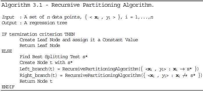
Regression trees are constructed using a recursive partitioning (RP) algorithm. This algorithm builds a tree by recursively splitting the training sample into smaller subsets. We give below a high level description of the algorithm. The RP algorithm receives as input a set of [math]\displaystyle{ n }[/math] data points, [math]\displaystyle{ D_t=\{\langle \mathbf{x_i},y_i\rangle\}^{n_t}_{i=1} }[/math], and if certain termination criteria are not met it generates a test node [math]\displaystyle{ t }[/math], whose branches are obtained by applying the same algorithm with two subsets of the input data points. These subsets consist of the cases that logically entail the split test [math]\displaystyle{ s^* }[/math] in the node [math]\displaystyle{ t }[/math], [math]\displaystyle{ D_{t_L}=\{\langle \mathbf{x_i},y_i\rangle\} \in D_t : \mathbf{x_i} \to s^*\} }[/math], and the remaining cases, [math]\displaystyle{ D_{t_R}=\{\langle \mathbf{x_i},y_i\rangle\} \in D_t : \mathbf{x_i} \not \to s^*\} }[/math]. At each node the best split test is chosen according to some local criterion, which means that this is a greedy hill-climbing algorithm.
The algorithm has three main components:
- A way to select a split test (the splitting rule).
- A rule to determine when a tree node is terminal (termination criterion).
- A rule for assigning a value to each terminal node.
In the following sections we present two different approaches to solve these problems. These alternatives try to minimise either the mean squared error or the mean absolute deviation of the resulting tree.
3.2 Least Squares Regression Trees
The most common method for building a regression model based on a sample of an unknown regression surface consists of trying to obtain the model parameters that minimise the least squares error criterion,
( ()) 2 , 1 å - b n i i i y r n x (3.2) where, n is the sample size; <xi , yi > is a data point ; and r(b, x_i ) is the prediction of the regression model r(b, x) for the case i i x , y .
As we have seen in Chapter 2 this criterion is used in many existing systems. RETIS (Karalic & Cestnik, 1991), M5 (Quinlan, 1992) and CART (Breiman et. al., 1984), all use the least squares (LS) criterion. To our knowledge the only tree induction system that is also able to use the mean absolute deviation is CART. The following theorem holds for the LS minimisation criterion:
THEOREM 3.1 The constant k that minimises the expected value of the squared error is the mean value of the target variable.
…
3.2.2 Splits on Continuous Variables
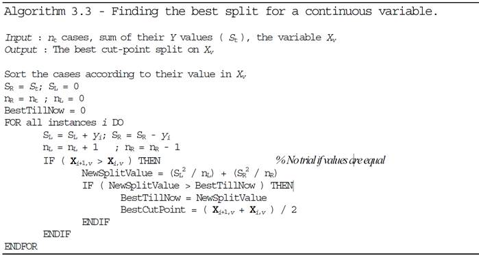
We will now present an algorithm that finds the best split for continuous variables using the results of Definition 3.2. Assuming that we have a set of nt cases whose sum of the Y values is St, Algorithm 3.3 obtains the best split on a continuous predictor variable Xv.
This algorithm has two main parts. The first consists of sorting the instances by the values of the variable being examined, which has an average complexity of O(nt log nt) using Quick Sort. This sorting operation is necessary for running through all trial cut-point values [26] in an efficient manner. We only need to try these cut-point values as they are the only ones that may change the value of the score given by Definition 3.2, because they modify the set of cases that go to the left and right branches. The second relevant part of the algorithm is the evaluation of all candidate splits. The number of trial splits is at most nt - 1 (if all instances have different value of the variable Xv). Without the equation given in Definition 3.2 we would have to calculate the “variance” of each of the partitions originated by the candidate split. This would involve passing through all data points (using the optimised formula of Equation 3.7) which is O(nt). This would lead to a worst case complexity of O(nt(nt -1)) for the second part of the algorithm. Our optimisation given by the formula in Definition 3.2 leads to a worst case complexity of O(nt - 1) as the “variance” calculation is avoided. Notice that this is only valid for the least squares error criterion that leads to the given simplification. If other criteria were used the complexity could be different particularly if no similar incremental algorithm could be found. With the existence of this fast and incremental method of computing the error gain of a split the complexity of the algorithm is dominated by the sorting operation.
…
References
,
| Author | volume | Date Value | title | type | journal | titleUrl | doi | note | year | |
|---|---|---|---|---|---|---|---|---|---|---|
| 1999 InductiveLearningofTreebasedReg | Luis Torgo | Inductive Learning of Tree-based Regression Models | 1999 |

