2015 TheUnreasonableEffectivenessofR
- (Karpathy, 2015) ⇒ Andrej Karpathy. (2015). “The Unreasonable Effectiveness of Recurrent Neural Networks.” In: Blog post 2015-05-21.
Subject Headings: Neural Character-level LM, RNNs, LSTMs.
Notes
Cited By
2015
- (Goldberg, 2015) ⇒ Yoav Goldberg. (2015). “The Unreasonable Effectiveness of Character-level Language Models (and Why RNNs Are Still Cool).” In: Blog Post.
- QUOTE: RNNs, LSTMs and Deep Learning are all the rage, and a recent blog post by Andrej Karpathy is doing a great job explaining what these models are and how to train them. It also provides some very impressive results of what they are capable of. This is a great post, and if you are interested in natural language, machine learning or neural networks you should definitely read it.
Quotes
Introduction
There’s something magical about Recurrent Neural Networks (RNNs). I still remember when I trained my first recurrent network for Image Captioning. Within a few dozen minutes of training my first baby model (with rather arbitrarily-chosen hyperparameters) started to generate very nice looking descriptions of images that were on the edge of making sense. Sometimes the ratio of how simple your model is to the quality of the results you get out of it blows past your expectations, and this was one of those times. What made this result so shocking at the time was that the common wisdom was that RNNs were supposed to be difficult to train (with more experience I’ve in fact reached the opposite conclusion). Fast forward about a year: I’m training RNNs all the time and I’ve witnessed their power and robustness many times, and yet their magical outputs still find ways of amusing me. This post is about sharing some of that magic with you.
We’ll train RNNs to generate text character by character and ponder the question “how is that even possible?”
By the way, together with this post I am also releasing code on Github that allows you to train character-level language models based on multi-layer LSTMs. You give it a large chunk of text and it will learn to generate text like it one character at a time. You can also use it to reproduce my experiments below. But we’re getting ahead of ourselves; What are RNNs anyway?
Recurrent Neural Networks
Sequences. Depending on your background you might be wondering: What makes Recurrent Networks so special? A glaring limitation of Vanilla Neural Networks (and also Convolutional Networks) is that their API is too constrained: they accept a fixed-sized vector as input (e.g. an image) and produce a fixed-sized vector as output (e.g. probabilities of different classes). Not only that: These models perform this mapping using a fixed amount of computational steps (e.g. the number of layers in the model). The core reason that recurrent nets are more exciting is that they allow us to operate over sequences of vectors: Sequences in the input, the output, or in the most general case both. A few examples may make this more concrete:
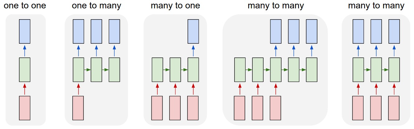
- Each rectangle is a vector and arrows represent functions (e.g. matrix multiply). Input vectors are in red, output vectors are in blue and green vectors hold the RNN's state (more on this soon). From left to right: (1) Vanilla mode of processing without RNN, from fixed-sized input to fixed-sized output (e.g. image classification). (2) Sequence output (e.g. image captioning takes an image and outputs a sentence of words). (3) Sequence input (e.g. sentiment analysis where a given sentence is classified as expressing positive or negative sentiment). (4) Sequence input and sequence output (e.g. Machine Translation: an RNN reads a sentence in English and then outputs a sentence in French). (5) Synced sequence input and output (e.g. video classification where we wish to label each frame of the video). Notice that in every case are no pre-specified constraints on the lengths sequences because the recurrent transformation (green) is fixed and can be applied as many times as we like.
As you might expect, the sequence regime of operation is much more powerful compared to fixed networks that are doomed from the get-go by a fixed number of computational steps, and hence also much more appealing for those of us who aspire to build more intelligent systems. Moreover, as we’ll see in a bit, RNNs combine the input vector with their state vector with a fixed (but learned) function to produce a new state vector. This can in programming terms be interpreted as running a fixed program with certain inputs and some internal variables. Viewed this way, RNNs essentially describe programs. In fact, it is known that RNNs are Turing-Complete in the sense that they can to simulate arbitrary programs (with proper weights). But similar to universal approximation theorems for neural nets you shouldn’t read too much into this. In fact, forget I said anything.
If training vanilla neural nets is optimization over functions, training recurrent nets is optimization over programs.
Sequential processing in absence of sequences. You might be thinking that having sequences as inputs or outputs could be relatively rare, but an important point to realize is that even if your inputs/outputs are fixed vectors, it is still possible to use this powerful formalism to process them in a sequential manner. For instance, the figure below shows results from two very nice papers from DeepMind. On the left, an algorithm learns a recurrent network policy that steers its attention around an image; In particular, it learns to read out house numbers from left to right (Ba et al.). On the right, a recurrent network generates images of digits by learning to sequentially add color to a canvas (Gregor et al.): Left: RNN learns to read house numbers. Right: RNN learns to paint house numbers.
The takeaway is that even if your data is not in form of sequences, you can still formulate and train powerful models that learn to process it sequentially. You’re learning stateful programs that process your fixed-sized data.
RNN computation. So how do these things work? At the core, RNNs have a deceptively simple API: They accept an input vector x and give you an output vector y. However, crucially this output vector’s contents are influenced not only by the input you just fed in, but also on the entire history of inputs you’ve fed in in the past. Written as a class, the RNN’s API consists of a single step function:
rnn = RNN() y = rnn.step(x) # x is an input vector, y is the RNN's output vector
The RNN class has some internal state that it gets to update every time step is called. In the simplest case this state consists of a single hidden vector h. Here is an implementation of the step function in a Vanilla RNN:
class RNN:
 # ...
 def step(self, x):
   # update the hidden state
   self.h = np.tanh(np.dot(self.W_hh, self.h) + np.dot(self.W_xh, x))
   # compute the output vector
   y = np.dot(self.W_hy, self.h)
   return y
The above specifies the forward pass of a vanilla RNN. This RNN’s parameters are the three matrices W_hh, W_xh, W_hy. The hidden state self.h is initialized with the zero vector. The np.tanh function implements a non-linearity that squashes the activations to the range [-1, 1]. Notice briefly how this works: There are two terms inside of the tanh: one is based on the previous hidden state and one is based on the current input. In numpy np.dot is matrix multiplication. The two intermediates interact with addition, and then get squashed by the tanh into the new state vector. If you’re more comfortable with math notation, we can also write the hidden state update as ht=tanh(Whhht−1+Wxhxt)
, where tanh is applied elementwise.
We initialize the matrices of the RNN with random numbers and the bulk of work during training goes into finding the matrices that give rise to desirable behavior, as measured with some loss function that expresses your preference to what kinds of outputs y you’d like to see in response to your input sequences x.
Going deep. RNNs are neural networks and everything works monotonically better (if done right) if you put on your deep learning that and start stacking models up like pancakes. For instance, we can form a 2-layer recurrent network as follows:
y1 = rnn1.step(x) y = rnn2.step(y1)
In other words we have two separate RNNs: One RNN is receiving the input vectors and the second RNN is receiving the output of the first RNN as its input. Except neither of these RNNs know or care - it’s all just vectors coming in and going out, and some gradients flowing through each module during backpropagation.
Getting fancy. I’d like to briefly mention that in practice most of us use a slightly different formulation than what I presented above called a Long Short-Term Memory (LSTM) network. The LSTM is a particular type of recurrent network that works slightly better in practice, owing to its more powerful update equation and some appealing backpropagation dynamics. I won’t go into details, but everything I’ve said about RNNs stays exactly the same, except the mathematical form for computing the update (the line self.h = ... ) gets a little more complicated. From here on I will use the terms “RNN/LSTM” interchangeably but all experiments in this post use an LSTM.
Character-Level Language Models
Okay, so we have an idea about what RNNs are, why they are super exciting, and how they work. We’ll now ground this in a fun application: We’ll train RNN character-level language models. That is, we’ll give the RNN a huge chunk of text and ask it to model the probability distribution of the next character in the sequence given a sequence of previous characters. This will then allow us to generate new text one character at a time.
As a working example, suppose we only had a vocabulary of four possible letters “helo”, and wanted to train an RNN on the training sequence “hello”. This training sequence is in fact a source of 4 separate training examples: 1. The probability of “e” should be likely given the context of “h”, 2. “l” should be likely in the context of “he”, 3. “l” should also be likely given the context of “hel”, and finally 4. “o” should be likely given the context of “hell”.
Concretely, we will encode each character into a vector using 1-of-k encoding (i.e. all zero except for a single one at the index of the character in the vocabulary), and feed them into the RNN one at a time with the step function. We will then observe a sequence of 4-dimensional output vectors (one dimension per character), which we interpret as the confidence the RNN currently assigns to each character coming next in the sequence. Here’s a diagram:
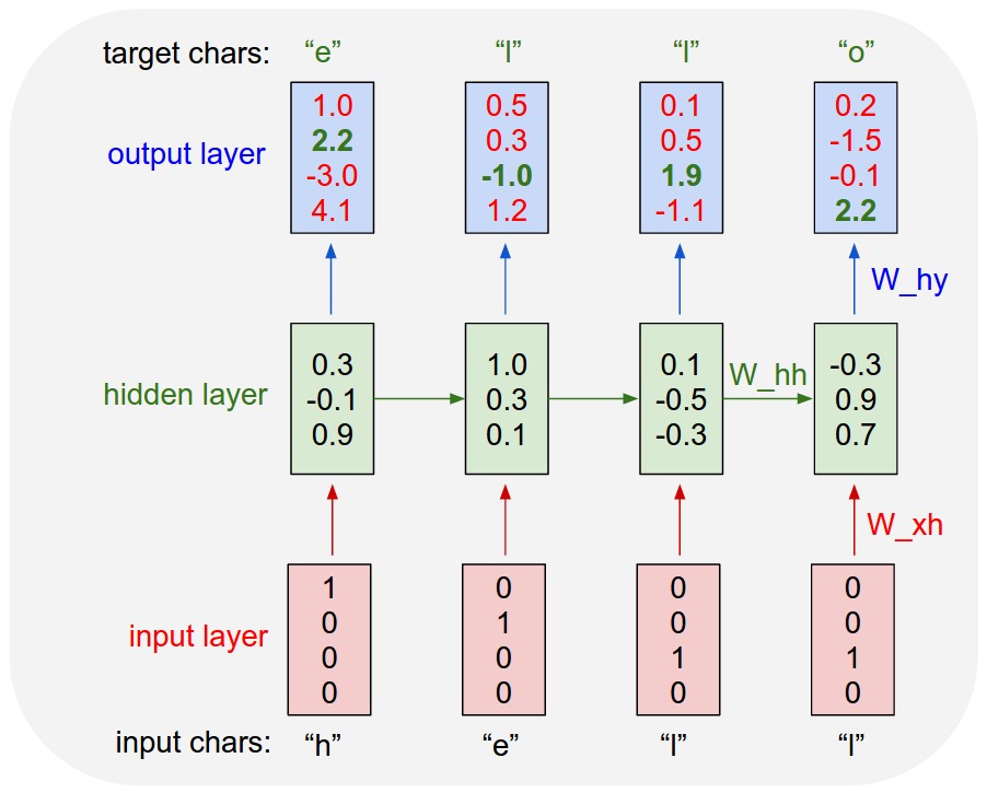
- An example RNN with 4-dimensional input and output layers, and a hidden layer of 3 units (neurons). This diagram shows the activations in the forward pass when the RNN is fed the characters "hell" as input. The output layer contains confidences the RNN assigns for the next character (vocabulary is "h,e,l,o"); We want the green numbers to be high and red numbers to be low.
For example, we see that in the first time step when the RNN saw the character “h” it assigned confidence of 1.0 to the next letter being “h”, 2.2 to letter “e”, -3.0 to “l”, and 4.1 to “o”. Since in our training data (the string “hello”) the next correct character is “e”, we would like to increase its confidence (green) and decrease the confidence of all other letters (red). Similarly, we have a desired target character at every one of the 4 time steps that we’d like the network to assign a greater confidence to. Since the RNN consists entirely of differentiable operations we can run the backpropagation algorithm (this is just a recursive application of the chain rule from calculus) to figure out in what direction we should adjust every one of its weights to increase the scores of the correct targets (green bold numbers). We can then perform a parameter update, which nudges every weight a tiny amount in this gradient direction. If we were to feed the same inputs to the RNN after the parameter update we would find that the scores of the correct characters (e.g. “e” in the first time step) would be slightly higher (e.g. 2.3 instead of 2.2), and the scores of incorrect characters would be slightly lower. We then repeat this process over and over many times until the network converges and its predictions are eventually consistent with the training data in that correct characters are always predicted next.
A more technical explanation is that we use the standard Softmax classifier (also commonly referred to as the cross-entropy loss) on every output vector simultaneously. The RNN is trained with mini-batch Stochastic Gradient Descent and I like to use RMSProp or Adam (per-parameter adaptive learning rate methods) to stabilize the updates.
Notice also that the first time the character “l” is input, the target is “l”, but the second time the target is “o”. The RNN therefore cannot rely on the input alone and must use its recurrent connection to keep track of the context to achieve this task.
At test time, we feed a character into the RNN and get a distribution over what characters are likely to come next. We sample from this distribution, and feed it right back in to get the next letter. Repeat this process and you’re sampling text! Lets now train an RNN on different datasets and see what happens.
To further clarify, for educational purposes I also wrote a minimal character-level RNN language model in Python/numpy. It is only about 100 lines long and hopefully it gives a concise, concrete and useful summary of the above if you’re better at reading code than text. We’ll now dive into example results, produced with the much more efficient Lua/Torch codebase.
References
;
| Author | volume | Date Value | title | type | journal | titleUrl | doi | note | year | |
|---|---|---|---|---|---|---|---|---|---|---|
| 2015 TheUnreasonableEffectivenessofR | Andrej Karpathy (1986-) | The Unreasonable Effectiveness of Recurrent Neural Networks | 2015 |