2017 RecurrentHighwayNetworks
- (Zilly et al., 2017) ⇒ Julian Georg Zilly, Rupesh Kumar Srivastava, Jan Koutník, and Jürgen Schmidhuber. (2017). “Recurrent Highway Networks.” In: Proceedings of the 34th International Conference on Machine Learning - Volume 70. arXiv:1607.03474
Subject Headings: Recurrent Highway Neural Network, Recurrent Neural Network, Deep Transition Function, Transtion Function, Nonlinear Transition Function, Gersgorin's Circle Theorem, Language Model.
Notes
Cited By
- Google Scholar: 232 Citations
- ACM DL: 5 Citations
- Semantic Scholar: 181 Citations
- NASA ADS: 79 Citations
Quotes
Abstract
Many sequential processing tasks require complex nonlinear transition functions from one step to the next. However, recurrent neural networks with " deep " transition functions remain difficult to train, even when using Long Short-Term Memory (LSTM) networks. We introduce a novel theoretical analysis of recurrent networks based on Gersgorin's circle theorem that illuminates several modeling and optimization issues and improves our understanding of the LSTM cell. Based on this analysis we propose Recurrent Highway Networks, which extend the LSTM architecture to allow step-to-step transition depths larger than one. Several language modeling experiments demonstrate that the proposed architecture results in powerful and efficient models. On the Penn Treebank corpus, solely increasing the transition depth from 1 to 10 improves word-level perplexity from 90.6 to 65.4 using the same number of parameters. On the larger Wikipedia datasets for character prediction (text8 and enwik8), RHNs outperform all previous results and achieve an entropy of 1.27 bits per character.
1. Introduction
Network depth is of central importance in the resurgence of neural networks as a powerful machine learning paradigm (Schmidhuber, 2015). Theoretical evidence indicates that deeper networks can be exponentially more efficient at representing certain function classes (see e.g. Bengio & LeCun (2007); Bianchini & Scarselli (2014) and references therein). Due to their sequential nature, Recurrent Neural Networks (RNNs; Robinson & Fallside, 1987; Werbos, 1988; Williams, 1989) have long credit assignment paths and so are deep in time. However, certain internal function mappings in modern RNNs composed of units grouped in layers usually do not take advantage of depth (Pascanu et al., 2013). For example, the state update from one time step to the next is typically modeled using a single trainable linear transformation followed by a non-linearity.
Unfortunately, increased depth represents a challenge when neural network parameters are optimized by means of error backpropagation (Linnainmaa, 1970; 1976; Werbos, 1982). Deep networks suffer from what are commonly referred to as the vanishing and exploding gradient problems (Hochreiter, 1991; Bengio et al., 1994; Hochreiter et al., 2001), since the magnitude of the gradients may shrink or explode exponentially during backpropagation. These training difficulties were first studied in the context of standard RNNs where the depth through time is proportional to the length of input sequence, which may have arbitrary size. The widely used Long Short-Term Memory (LSTM; Hochreiter & Schmidhuber, 1997; Gers et al., 2000) architecture was introduced to specifically address the problem of vanishing / exploding gradients for recurrent networks.
The vanishing gradient problem also becomes a limitation when training very deep feedforward networks. Highway Layers (Srivastava et al., 2015b) based on the LSTM cell addressed this limitation enabling the training of networks even with hundreds of stacked layers. Used as feedforward connections, these layers were used to improve performance in many domains such as speech recognition (Zhang et al., 2016) and language modeling (Kim et al., 2015; Jozefowicz et al., 2016), and their variants called Residual networks have been widely useful for many Computer Vision problems (He et al., 2015).
In this paper we first provide a new mathematical analysis of RNNs which offers a deeper understanding of the strengths of the LSTM cell. Based on these insights, we introduce LSTM networks that have long credit assignment paths not just in time but also in space (per time step), called Recurrent Highway Networks or RHNs. Unlike previous work on deep RNNs, this model incorporates Highway layers inside the recurrent transition, which we argue is a superior method of increasing depth. This enables the use of substantially more powerful and trainable sequential models efficiently, significantly outperforming existing architectures on widely used benchmarks.
2. Related Work on Deep Recurrent Transitions
In recent years, a common method of utilizing the computational advantages of depth in recurrent networks is slacking recurrent layers (Schmidhuber, 1992), which is analogous to using multiple hidden layers in feedforward networks. Training stacked RNNs naturally requires credit assignment across both space and time which is difficult in practice. These problems have been recently addressed by architectures utilizing LSTM-based transformations for stacking (Zhang et al., 2016; Kalchbrenner et al., 2015).
A general method to increase the depth of the step-to-step recurrent state transition (the recurrence depth) is to let an RNN tick for several micro time steps per step of the sequence (Schmidhuber, 1991; Srivastava et al., 2013; Graves, 2016). This method can adapt the recurrence depth to the problem, but the RNN has to learn by itself which parameters to use for memories of previous events and which for standard deep nonlinear processing. It is notable that while Graves (2016) reported improvements on simple algorithmic tasks using this method, no performance improvements were obtained on real world data.
Pascanu et al. (2013) proposed to increase the recurrence depth by adding multiple non-linear layers to the recurrent transition, resulting in Deep Transition RNNs (DT-RNNs) and Deep Transition RNNs with Skip connections (DT(S)-RNNs). While being powerful in principle, these architectures are seldom used due to exacerbated gradient propagation issues resulting from extremely long credit assignment paths [1]. In related work Chung et al. (2015) added extra connections between all states across consecutive time steps in a stacked RNN, which also increases recurrence depth. However, their model requires many extra connections with increasing depth, gives only a fraction of states access to the largest depth, and still faces gradient propagation issues along the longest paths.
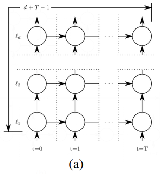
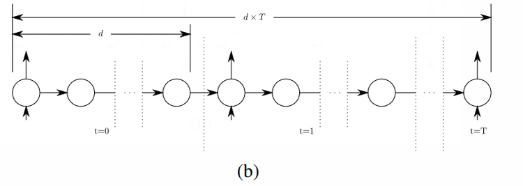
Compared to stacking recurrent layers, increasing the recurrence depth can add significantly higher modeling power to an RNN. Figure 1 illustrates that stacking [math]\displaystyle{ d }[/math] RNN layers allows a maximum credit assignment path length (number of non-linear transformations) of [math]\displaystyle{ d + T - 1 }[/math] between hidden states which are [math]\displaystyle{ T }[/math] time steps apart, while a recurrence depth of [math]\displaystyle{ d }[/math] enables a maximum path length of [math]\displaystyle{ d \times T }[/math]. While this allows greater power and efficiency using larger depths, it also explains why such architectures are much more difficult to train compared to stacked RNNs. In the next sections, we address this problem head on by focusing on the key mechanisms of the LSTM and using those to design RHNs, which do not suffer from the above difficulties.
Figure 1: Comparison of (a) stacked RNN with depth [math]\displaystyle{ d }[/math] and (b) Deep Transition RNN of recurrence depth [math]\displaystyle{ d }[/math], both operating on a sequence of [math]\displaystyle{ T }[/math] time steps. The longest credit assignment path between hidden states [math]\displaystyle{ T }[/math] time steps is [math]\displaystyle{ d \times T }[/math] for Deep Transition RNNs.
- ↑ Training of our proposed architecture is compared to these models in subsection 5.1.
3. Revisiting Gradient Flow in Recurrent Networks
Let [math]\displaystyle{ \mathcal{L} }[/math] denote the total loss for an input sequence of length [math]\displaystyle{ T }[/math]. Let [math]\displaystyle{ x^{[t]} \in \mathbb{R}^m }[/math] and [math]\displaystyle{ y^{[t]} \in \mathbb{R}^n }[/math] represent the output of a standard RNN at time [math]\displaystyle{ t }[/math], [math]\displaystyle{ W \in \mathbb{R}^{n\times m} }[/math] and [math]\displaystyle{ R \in \mathbb{R}^{n\times n} }[/math] the input and recurrent weight matrices, [math]\displaystyle{ b \in R^n }[/math] a bias vector and [math]\displaystyle{ f }[/math] a point-wise non-linearity. Then [math]\displaystyle{ y^{[t]} = f \left( Wx^{[t]} + Ry^{[t-1]} + b\right) }[/math] describes the dynamics of a standard RNN. The derivative of the loss [math]\displaystyle{ \mathcal{L} }[/math] with respect to parameters [math]\displaystyle{ }[/math] of a network can be expanded using the chain rule:
[math]\displaystyle{ \dfrac{\partial \mathcal{L}}{\partial \theta} = \displaystyle\sum_{1 \leq t_2 \leq T}\dfrac{\partial \mathcal{L}^{[t_2]}}{\partial \theta} = \displaystyle\sum_{1 \leq t_2 \leq T} \displaystyle\sum_{1 \leq t_1 \leq t_2} \dfrac{\partial \mathcal{L}^{[t_2]}}{\partial y^{[t_2]}}\dfrac{\partial y^{[t_2]}}{\partial y^{[t_1]}}\dfrac{\partial y^{[t_2]}}{\partial \theta} \quad }[/math] (1)
The Jacobian matrix [math]\displaystyle{ \dfrac{\partial y^{[t_2]}}{\partial y^{[t_1]}} }[/math], the key factor for the transport of the error from time step [math]\displaystyle{ t_2 }[/math] to time step [math]\displaystyle{ t_1 }[/math], is obtained by chaining the derivatives across all time steps:
[math]\displaystyle{ \dfrac{\partial y^{[t_2]}}{\partial y^{[t_1]}} = \displaystyle\prod_{t_1 \leq t \leq t_2}\dfrac{\partial y^{[t]}}{\partial y^{[t-1]}} = \displaystyle\prod_{t_1 \leq t \leq t_2} R^{\top}\mathrm{diag}[f'(R y^{[t-1]})]\quad }[/math] (2)
where the input and bias have been omitted for simplicity. We can now obtain conditions for the gradients to vanish or explode. Let [math]\displaystyle{ A := \dfrac{\partial y^{[t]}}{\partial y^{[t-1]}} }[/math] be the temporal Jacobian, [math]\displaystyle{ \gamma }[/math] be a maximal bound on [math]\displaystyle{ f’(Ry^{[t-1]}) }[/math] and [math]\displaystyle{ \sigma_{max} }[/math] be the largest singular value of [math]\displaystyle{ R^{top} }[/math]. Then the norm of the Jacobian satisfies:
which together with (2) provides the conditions for vanishing gradients ([math]\displaystyle{ \gamma \sigma_{max}\lt 1 }[/math]). Note that [math]\displaystyle{ \gamma }[/math] depends on the activation function [math]\displaystyle{ f }[/math], e.g. [math]\displaystyle{ |tanh'(x)| \leq 1 }[/math], [math]\displaystyle{ |\sigma'(x)|\leq \dfrac{1}{4} }[/math], [math]\displaystyle{ \forall x \in \mathbb{R} }[/math], where [math]\displaystyle{ \sigma }[/math] is a logistic sigmoid. Similarly, we can show that if the spectral radius [math]\displaystyle{ \rho }[/math] of [math]\displaystyle{ A }[/math] is greater than [math]\displaystyle{ 1 }[/math], exploding gradients will emerge since [math]\displaystyle{ \parallel A \parallel \geq \rho }[/math].
This description of the problem in terms of largest singular values or the spectral radius sheds light on boundary conditions for vanishing and exploding gradients yet does not illuminate how the eigenvalues are[distributed overall. By applying the Gersgorin circle theorem we are able to provide further insight into this problem.
==== Gersgorin circle theorem (GCT) (Gersgorin, 1931) ==== For any square matrix [math]\displaystyle{ A \in \mathbb{R}^{m\times n} }[/math],
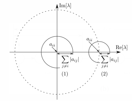
i.e., the eigenvalues of matrix [math]\displaystyle{ A }[/math], comprising the spectrum of [math]\displaystyle{ A }[/math], are located within the union of the complex circles centered around the diagonal values [math]\displaystyle{ a_{ii} }[/math] of [math]\displaystyle{ A }[/math] with radius [math]\displaystyle{ \displaystyle\sum_{j=1, j\neq i}^n |a_{ij}| }[/math] equal to the sum of the absolute values of the non-diagonal entries in each row of [math]\displaystyle{ A }[/math]. Two example Gersgorin circles referring to differently initialized RNNs are depicted in Figure 2.
|
Using GCT we can understand the relationship between the entries of [math]\displaystyle{ R }[/math] and the possible locations of the eigenvalues of the Jacobian. Shifting the diagonal values [math]\displaystyle{ a_{ii} }[/math] shifts the possible locations of eigenvalues. Having large off-diagonal entries will allow for a large spread of eigenvalues. Small off-diagonal entries yield smaller radii and thus a more confined distribution of eigenvalues around the diagonal entries [math]\displaystyle{ a_{ii} }[/math].
Let us assume that matrix [math]\displaystyle{ R }[/math] is initialized with a zero-mean Gaussian distribution. We can then infer the following:
- If the values of [math]\displaystyle{ R }[/math] are initialized with a standard deviation close to 0, then the spectrum of [math]\displaystyle{ A }[/math], which is largely dependent on [math]\displaystyle{ R }[/math], is also initially centered around 0. An example of a Gersgorin circle that could then be corresponding to a row of [math]\displaystyle{ A }[/math] is circle (1) in Figure 2. The magnitude of most of [math]\displaystyle{ A }[/math]’s eigenvalues [math]\displaystyle{ |\lambda_i| }[/math] are initially likely to be substantially smaller than 1. Additionally, employing the commonly used [math]\displaystyle{ L_1/L_2 }[/math] weight regularization will also limit the magnitude of the eigenvalues.
- Alternatively, if entries of [math]\displaystyle{ R }[/math] are initialized with a large standard deviation, the radii of the Gersgorin circles corresponding to [math]\displaystyle{ A }[/math] increase. Hence, [math]\displaystyle{ A }[/math]’s spectrum may possess eigenvalues with norms greater 1 resulting in exploding gradients. As the radii are summed over the size of the matrix, larger matrices will have an associated larger circle radius. In consequence, larger matrices should be initialized with correspondingly smaller standard deviations to avoid exploding gradients.
In general, unlike variants of LSTM, other RNNs have no direct mechanism to rapidly regulate their Jacobian eigenvalues across time steps, which we hypothesize can be efficient and necessary for learning complex sequence processing.
Le et al. (2015) proposed to initialize [math]\displaystyle{ R }[/math] with an identity matrix and small random values on the off-diagonals. This changes the situation depicted by GCT the result of the identity initialization is indicated by circle (2) in Figure 2. Initially, since [math]\displaystyle{ a_{ii}= 1 }[/math], the spectrum described in GCT is centered around 1, ensuring that gradients are less likely to vanish. However, this is not a flexible remedy. During training some eigenvalues can easily become larger than one, resulting in exploding gradients. We conjecture that due to this reason, extremely small learning rates were used by Le et al. (2015).
4. Recurrent Highway Networks (RHN)
Highway layers (Srivastava et al., 2015a) enable easy training of very deep feedforward networks through the use of adaptive computation. $\mathbf{h}=H\left(\mathbf{x}, \mathbf{W}_{H}\right), \mathbf{t}= T\left(\mathbf{x}, \mathbf{W}_{T}\right), \mathbf{c}=C\left(\mathbf{x}, \mathbf{W}_{C}\right)$ be outputs of nonlinear transforms $H$ , $T$ and $C$ with associated weight matrices (including biases) $\mathbf{W}_{H,T,C}$. $T$ and $C$ typically utilize a sigmoid ($\sigma$) nonlinearity and are referred to as the transform and the carry gates since they regulate the passing of the transformed input via $H$ or the carrying over of the original input $x$. The Highway layer computation is defined as
| $\mathbf{y}=\mathbf{h} \cdot \mathbf{t}+\mathbf{x} \cdot \mathbf{c}$ | (5) |
where "-" denotes element-wise multiplication.
Recall that the recurrent state transition in a standard RNN is described by $\mathbf{y}^{[t]}=f\left(\mathbf{W} \mathbf{x}^{[t]}+\mathbf{R} \mathbf{y}^{[t-1]}+\mathbf{b}\right)$. We propose to construct a Recurrent Highway Network (RHN) layer with one or multiple Highway layers in the recurrent state transition (equal to the desired recurrence depth). Formally, let $\mathbf{W}_{H , T , C} \in \mathbb{R}^{n \times m}$ and $\mathbf{R}_{H , T , C} \in \mathbb{R}^{n \times n}$ represent the weights matrices of the $H$ nonlinear transform and the $T$ and $C$ gates at layer $\ell \in \{1, \cdots , L\}$. The biases are denoted by $\mathbf{b}_{H_{\ell} , T_{\ell} , C_{\ell}} \in \mathbb{R}^{n}$ and let $s_{\ell}$ denote the intermediate output at layerwith $s_0^{[t]} = y^{[t−1]}$. Then an RHN layer with a recurrence depth of $L$ is described by
| $\mathbf{s}_{\ell}^{[t]}=\mathbf{h}_{\ell}^{[t]} \cdot \mathbf{t}_{\ell}^{[t]}+\mathbf{s}_{\ell-1}^{[t]} \cdot \mathbf{c}_{\ell}^{[t]}$ | (6) |
where
| $\mathbf{h}_{\ell}^{[t]}=\tanh \left(\mathbf{W}_{H} \mathbf{x}^{[t]} \mathbb{I}_{\{\ell=1\}}+\mathbf{R}_{H_{\ell}} \mathbf{s}_{\ell-1}^{[t]}+\mathbf{b}_{H_{\ell}}\right)$, | (7) |
| $\mathbf{t}_{\ell}^{[t]}= \sigma\left(\mathbf{W}_{T} \mathbf{x}^{[t]} \mathbb{I}_{\{\ell=1\}}+\mathbf{R}_{T_{\ell}} \mathbf{s}_{\ell-1}^{[t]}+\mathbf{b}_{T_{\ell}}\right)$ | (8) |
| $\mathbf{c}_{\ell}^{[t]}= \sigma\left(\mathbf{W}_{C} \mathbf{x}^{[t]} \mathbb{I}_{\{\ell=1\}}+\mathbf{R}_{C_{\ell}} \mathbf{s}_{\ell-1}^{[t]}+\mathbf{b}_{C_{\ell}}\right)$ | (9) |
and $\mathbb{I}_{\{\}}$ is the indicator function.
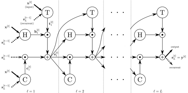
A schematic illustration of the RHN computation graph is shown in Figure 3. The output of the RHN layer is the output of the $L$th Highway layer i.e. $y^{[t]} =s_{L}^{[t]}$.
|
Note that $x^{[t]}$ is directly transformed only by the first Highway layer ($\ell = 1$) in the recurrent transition[1] and for this layer sill is the RHN layer's output of the previous time step. Subsequent Highway layers only process the outputs of the previous layers. Dotted vertical lines in Figure 3 separate multiple Highway layers in the recurrent transition.
For conceptual clarity, it is important to observe that an RHN layer with $L = 1$ is essentially a basic variant of an LSTM layer. Similar to other variants such as GRU (Cho et al., 2014) and those studied by Greff et al. (2015) and Jozefowicz et al. (2015), it retains the essential components of the LSTM multiplicative gating units controlling the flow of information through self-connected additive cells. However, an RHN layer naturally extends to $L > 1$, extending the LSTM to model far more complex state transitions. Similar to Highway and LSTM layers, other variants can be constructed without changing the basic principles, for example by fixing one or both of the gates to always be open, or coupling the gates as done for the experiments in this paper.
The simpler formulation of RHN layers allows for an analysis similar to standard RNNs based on GCT. Omitting the inputs and biases, the temporal Jacobian $\mathbf{A}=\partial \mathbf{y}^{[t]} / \partial \mathbf{y}^{[t-1]}$ for an RHN layer with recurrence depth of 1 ($\mathbf{y}^{[t]}=\mathbf{h}^{[t]} \cdot \mathbf{t}^{[t]}+\mathbf{y}^{[t-1]} \cdot \mathbf{c}^{[t]}$) is given by
|
$\mathbf{A}=\operatorname{diag}\left(\mathbf{c}^{[t]}\right)+\mathbf{H}^{\prime} \operatorname{diag}\left(\mathbf{t}^{[t]}\right)+\mathbf{C}^{\prime} \operatorname{diag}\left(\mathbf{y}^{[t-1]}\right)+\mathbf{T}^{\prime} \operatorname{diag}\left(\mathbf{h}^{[t]}\right)$ |
(10) |
where
| $\mathbf{H}^{\prime}=\mathbf{R}_{H}^{\top} \operatorname{diag}\left[\tanh ^{\prime}\left(\mathbf{R}_{H} \mathbf{y}^{[t-1]}\right)\right]$, | (11) |
| $\mathbf{T}^{\prime}=\mathbf{R}_{T}^{\top} \operatorname{diag}\left[\sigma^{\prime}\left(\mathbf{R}_{T} \mathbf{y}^{[t-1]}\right)\right]$ | (12) |
| $\mathbf{C}^{\prime}=\mathbf{R}_{C}^{\top} \operatorname{diag}\left[\sigma^{\prime}\left(\mathbf{R}_{C} \mathbf{y}^{[t-1]}\right)\right]$ | (13) |
and has a spectrum of:
|
$\operatorname{spec}(\mathbf{A}) \subset \bigcup_{i \in\{1, \ldots, n\}}\left\{\lambda \in \mathbb{C} \mid \| \lambda-\mathbf{c}_{i}^{[t]}-\mathbf{H}_{i i}^{\prime} \mathbf{t}_{i}^{[t]}-\mathbf{C}_{i i}^{\prime} \mathbf{y}_{i}^{[t-1]}-\mathbf{T}_{i i}^{\prime} \mathbf{h}_{i}^{[t]} \|_{\mathbb{C}} \leq \sum_{j=1, j \neq i}^{n}\left|\mathbf{H}_{i j}^{\prime} \mathbf{t}_{i}^{[t]}+\mathbf{C}_{i j}^{\prime} \mathbf{y}_{i}^{[t-1]}+\mathbf{T}_{i j}^{\prime} \mathbf{h}_{i}^{[t]}\right|\right\} $ |
(14) |
Equation 14 captures the influence of the gates on the eigenvalues of $\mathbf{A}$. Compared to the situation for standard RNN, it can be seen that an RHN layer has more flexibility in adjusting the centers and radii of the Gersgorin circles. In particular, two limiting cases can be noted. If all carry gates are fully open and transform gates are fully closed, we have $\mathbf{c =1_n}$,, $\mathbf{t = 0_n}$ and $T' = C'=0_{n\times n}$ (since $\sigma$ is saturated). This results in
| $\mathbf{c}=\mathbf{1}_{n}, \quad \mathbf{t}=\mathbf{0}_{n} \Rightarrow \lambda_{i}=1 \quad \forall i \in\{1, \ldots, n\}$ | (15) |
i.e. all eigenvalues are set to 1 since the Gersgorin circle radius is shrunk to 0 and each diagonal entry is set to $\mathbf{c_i = 1}$. In the other limiting case, if $\mathbf{c = 0_n}$ and $\mathbf{t=1_n}$, then the eigenvalues are simply those of $\mathbf{H}'$. As the gates vary between 0 and 1, each of the eigenvalues of $\mathbf{A}$ can be dynamically adjusted to any combination of the above limiting behaviors.
The key takeaways from the above analysis are as follows. Firstly, GCT allows us to observe the behavior of the full spectrum of the temporal Jacobian, and the effect of gating units on it. We expect that for learning multiple temporal dependencies from real-world data efficiently, it is not sufficient to avoid vanishing and exploding gradients. The gates in RHN layers provide a more versatile setup for dynamically remembering, forgetting and transforming information compared to standard RNNs. Secondly, it becomes clear that through their effect on the behavior of the Jacobian, highly non-linear gating functions can facilitate learning through rapid and precise regulation of the network dynamics. Depth is a widely used method to add expressive power to functions, motivating us to use multiple layers of $H$, $T$ and $C$ transformations. In this paper we opt for extending RHN layers to $L > 1$ using Highway layers in favor of simplicity and ease of training. However, we expect that in some cases stacking plain layers for these transformations can also be useful. Finally, the analysis of the RHN layer's flexibility in controlling its spectrum furthers our theoretical understanding of LSTM and Highway networks and their variants. For feedforward Highway networks, the Jacobian of the layer transformation ($\partial \mathbf{y}/\partial \mathbf{x}$) takes the place of the temporal Jacobian in the above analysis. Each Highway layer allows increased flexibility in controlling how various components of the input are transformed or carried. This flexibility is the likely reason behind the performance improvement from Highway layers even in cases where network depth is not high (Kim et al., 2015).
5. Experiments
Setup: In this work, the carry gate was coupled to the transform gate by setting $C (\cdot)= \mathbf{1_n} - T (\cdot)$ similar to the suggestion for Highway networks. This coupling is also used by the GRU recurrent architecture. It reduces model size for a fixed number of units and prevents an unbounded blow-up of state values leading to more stable training, but imposes a modeling bias which may be sub-optimal for certain tasks (Greff et al., 2015; Jozefowicz et al., 2015). An output non-linearity similar to LSTM networks could alternatively be used to combat this issue. For optimization and Wikipedia experiments, we bias the transform gates towards being closed at the start of training. All networks use a single hidden RHN layer since we are only interested in studying the influence of recurrence depth, and not of stacking multiple layers, which is already known to be useful. Detailed configurations for all experiments are included in the supplementary material.
Regularization of RHNs: Like all RNNs, suitable regularization can be essential for obtaining good generalization with RHNs in practice. We adopt the regularization technique proposed by Gal (2015), which is an interpretation of dropout based on approximate variational inference. RHNs regularized by this technique are referred to as variational RHNs. For the Penn Treebank word-level language modeling task, we report results both with and without weight-tying (WT) of input and output mappings for fair comparisons. This regularization was independently proposed by Inan & Khosravi (2016) and Press & Wolf (2016).
5.1. Optimization
RHN is an architecture designed to enable the optimization of recurrent networks with deep transitions. Therefore, the primary experimental verification we seek is whether RHNs with higher recurrence depth are easier to optimize compared to other alternatives, preferably using simple gradient based methods.
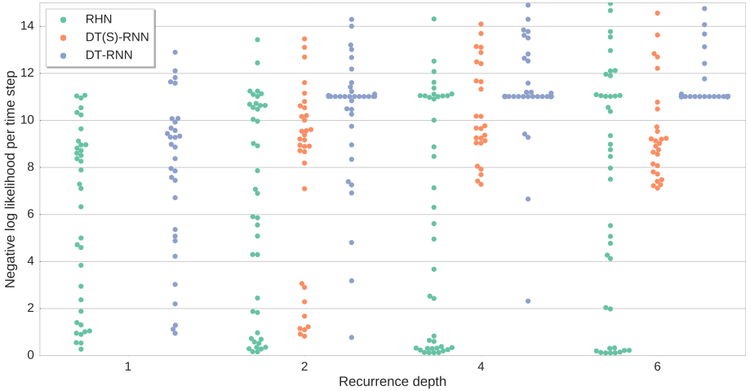
We compare optimization of RHNs to DT-RNNs and DT(S)-RNNs (Pascanu et al., 2013). Networks with recurrence depth of 1, 2, 4 and 6 are trained for next step prediction on the JSB Chorales polyphonic music prediction dataset (Boulanger-Lewandowski et al., 2012). Network sizes are chosen such that the total number of network parameters increases as the recurrence depth increases, but remains the same across architectures. A hyperparameter search is then conducted for SGD-based optimization of each architecture and depth combination for fair comparisons. In the absence of optimization difficulties, larger networks should reach a similar or better loss value compared to smaller networks. However, the swarm plot in Figure 4 shows that both DT-RNN and DT(S)-RNN become considerably harder to optimize with increasing depth. Similar to feedforward Highway networks, increasing the recurrence depth does not adversely affect optimization of RHNs.
|
5.2. Sequence Modeling
5.2.1. PENN TREEBANK
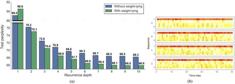
To examine the effect of recurrence depth we train RHNs with fixed total parameters (32M) and recurrence depths ranging from 1 to 10 for word level language modeling on the Penn TreeBank dataset (Marcus et al., 1993) preprocessed by Mikolov et al. (2010). The same hyperparameters are used to train each model. For each depth, we show the test set perplexity of the best model based on performance on the validation set in Figure 5(a). Additionally we also report the results for each model trained with WT regularization. In both cases the test score improves as the recurrence depth increases from 1 to 10. For the best 10 layer model, reducing the weight decay further improves the results to 67.9 /65.4 validation/test perplexity.
As the recurrence depth increases from 1 to 10 layers the "width" of the network decreases from 1275 to 830 units since the number of parameters was kept fixed. Thus, these results demonstrate that even for small datasets utilizing parameters to increase depth can yield large benefits even though the size of the RNN "state" is reduced. Table 1 compares our result with the best published results on this dataset. The directly comparable baseline is Variational LSTM+WT, which only differs in network architecture and size from our models. RHNs outperform most single models as well as all previous ensembles, and also benefit from WT regularization similar to LSTMs. Solely the yet to be analyzed architecture found through reinforcement learning and hyperparamater search by Zoph & Le (2016) achieves better results.
|
5.2.2. WIKIPEDIA
The task for this experiment is next symbol prediction on the challenging Hutter Prize Wikipedia datasets text8 and enwik8 (Hutter, 2012) with 27 and 205 unicode symbols in total, respectively. Due to its size (100 M characters in total) and complexity (inclusion of Latin/non-Latin alphabets, XML markup and various special characters for enwik8) these datasets allow us to stress the learning and generalization capacity of RHNs. We train various variational RHNs with recurrence depth of 5 or 10 and 1000 or 1500 units per hidden layer, obtaining state-of-the-art results. On text8 a validation/test set BPC of 1.19/1.27 for a model with 1500 units and recurrence depth 10 is achieved. Similarly, on enwik8 a validation / test set BPC of 1.26/1.27 is achieved for the same model and hyperparameters. The only difference between the models is the size of the embedding layer, which is set to the size of the character set. Table 2 and Table 3 show that RHNs outperform the previous best models on text8 and enwik8 with significantly fewer total parameters. A more detailed description of the networks is provided in the supplementary material.
| Model | BPC | Size |
|---|---|---|
| Grid-LSTM (Kalchbrenner et al., 2015) | 1.47 | 17 M |
| MI-LSTM (Wu et al., 2016) | 1.44 | 17 M |
| mLSTM (Krause et al., 2016) | 1.42 | 21 M |
| LN HyperNetworks (Ha et al., 2016) | 1.34 | 27 M |
| LN HM-LSTM (Chung et al., 2016) | 1.32 | 35 M |
| RHN - Rec. depth 5 | 1.31 | 23 M |
| RHN - Rec. depth 10 | 1.30 | 21 M |
| Large RHN - Rec. depth 10 | 1.27 | 46 M |
| Model | BPC | Size |
|---|---|---|
| MI-LSTM (Wu et al., 2016) | 1.44 | 17 M |
| mLSTM (Krause et al., 2016) | 1.40 | 10 M |
| BN LSTM (Cooijmans et al., 2016) | 1.36 | 16 M |
| HM-LSTM (Chung et al., 2016) | 1.32 | 35 M |
| LN HM-LSTM (Chung et al., 2016) | 1.29 | 35 M |
| RHN - Rec. depth 10 | 1.29 | 20 M |
| Large RHN - Rec. depth 10 | 1.27 | 45 M |
6. Analysis
We analyze the inner workings of RHNs through inspection of gate activations, and their effect on network performance. For the RHN with a recurrence depth of six optimized on the JSB Chorales dataset (subsection 5.1), Figure 5 (b) shows the mean transform gate activity in each layer over time steps for 4 example sequences. We note that while the gates are biased towards zero (white) at initialization, all layers are utilized in the trained network. The gate activity in the first layer of the recurrent transition is typically high on average, indicating that at least one layer of recurrent transition is almost always utilized. Gates in other layers have varied behavior, dynamically switching their activity over time in a different way for each sequence.
Similar to the feedforward case, the Highway layers in RHNs perform adaptive computation, i.e. the effective amount of transformation is dynamically adjusted for each sequence and time step. Unlike the general methods mentioned in section 2, the maximum depth is limited to the recurrence depth of the RHN layer. A concrete description of such computations in feedforward networks has recently been offered in terms of learning unrolled iterative estimation (Greff et al., 2016). This description carries over to RHNs the first layer in the recurrent transition computes a rough estimation of how the memory state should change given new information. The memory state is then further refined by successive layers resulting in better estimates.
The contributions of the layers towards network performance can be quantified through a lesioning experiment (Srivastava et al., 2015a). For one Highway layer at a time, all the gates are pushed towards carry behavior by setting the bias to a large negative value, and the resulting loss on the training set is measured. The change in loss due to the biasing of each layer measures its contribution to the network performance. For RHNs, we find that the first layer in the recurrent transition contributes much more to the overall performance compared to others, but removing any layer in general lowers the performance substantially due to the recurrent nature of the network. A plot of obtained results is included in the supplementary material.
7. Conclusion
We developed a new analysis of the behavior of RNNs based on the Gersgorin Circle Theorem. The analysis provided insights about the ability of gates to variably influence learning in a simplified version of LSTMs. We introduced Recurrent Highway Networks, a powerful new model designed to take advantage of increased depth in the recurrent transition while retaining the ease of training of LSTMs. Experiments confirmed the theoretical optimization advantages as well as improved performance on well known sequence modeling tasks.
Acknowledgements
This research was partially supported by the H2020 project “Intuitive Natural Prosthesis UTilization” (INPUT; #687795) and SNSF grant “Advanced Reinforcement Learning” (#156682). We thank Klaus Greff, Sjoerd van Steenkiste, Wonmin Byeon and Bas Steunebrink for many insightful discussions. We are grateful to NVIDIA Corporation for providing a DGX—l computer to IDSIA as part of the Pioneers of AI Research award.
Footnotes
- ↑ This is not strictly necessary, but simply a convenient choice.
References
BibTeX
@inproceedings{2017_RecurrentHighwayNetworks,
  author    = {Julian Georg Zilly and
               Rupesh Kumar Srivastava and
               Jan Koutnik and
               Jurgen Schmidhuber},
  editor    = {Doina Precup and
               Yee Whye Teh},
  title     = {Recurrent Highway Networks},
  booktitle = {Proceedings of the 34th International Conference on Machine Learning (ICML 2017)},
  series    = {Proceedings of Machine Learning Research},
  volume    = {70},
  pages     = {4189--4198},
  publisher = {PMLR},
  year      = {2017},
  url       = {http://proceedings.mlr.press/v70/zilly17a.html},
}
| Author | volume | Date Value | title | type | journal | titleUrl | doi | note | year | |
|---|---|---|---|---|---|---|---|---|---|---|
| 2017 RecurrentHighwayNetworks | Jürgen Schmidhuber Julian Georg Zilly Rupesh Kumar Srivastava Jan Koutník | Recurrent Highway Networks | 2017 |
