2018 NeuralFactorGraphModelsforCross

• (Malaviya et al., 2018) ⇒ Chaitanya Malaviya, Matthew R. Gormley, and Graham Neubig. (2018). “Neural Factor Graph Models for Cross-lingual Morphological Tagging .” In: arXiv:1805.04570 Journal.

Subject Headings: Morphological Analysis, Factorial Conditional Random Field.

Cited By

• http://scholar.google.com/scholar?q=%222018%22+Neural+Factor+Graph+Models+for+Cross-lingual+Morphological+Tagging+

Quotes

Abstract

Morphological analysis involves predicting the syntactic traits of a word (e.g. {POS:Noun, Case:Acc, Gender:Fem}). Previous work in morphological tagging improves performance for low-resource languages (LRLs) through cross-lingual training with a high-resource language (HRL) from the same family, but is limited by the strict, often false, assumption that tag sets exactly overlap between the HRL and LRL. In this paper we propose a method for cross-lingual morphological tagging that aims to improve information sharing between languages by relaxing this assumption. The proposed model uses factorial conditional random fields with neural network potentials, making it possible to (1) utilize the expressive power of neural network representations to smooth over superficial differences in the surface forms, (2) model pairwise and transitive relationships between tags, and (3) accurately generate tag sets that are unseen or rare in the training data. Experiments on four languages from the Universal Dependencies Treebank demonstrate superior tagging accuracies over existing cross-lingual approaches .

1 Introduction

Morphological analysis (Hajič and Hladká (1998), Oflazer and Kuruöz (1994), inter alia) is the task of predicting fine-grained annotations about the syntactic properties of tokens in a language such as part-of-speech, case, or tense. For instance, in Figure 1, the given Portuguese sentence is labeled with the respective morphological tags such as Gender and its label value Masculine.

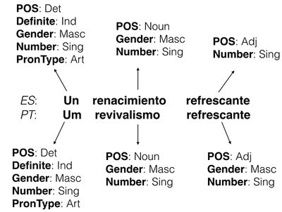
Figure 1: Morphological tags for a UD sentence in Portuguese and a translation in Spanish

The accuracy of morphological analyzers is paramount, because their results are often a first step in the NLP pipeline for tasks such as transla- tion (Vylomova et al., 2017; Tsarfaty et al., 2010) and parsing (Tsarfaty et al., 2013), and errors in the upstream analysis may cascade to the down- stream tasks. One difficulty, however, in creating these taggers is that only a limited amount of anno- tated data is available for a majority of the world’s languages to learn these morphological taggers. Fortunately, recent efforts in morphological an- notation follow a standard annotation schema for these morphological tags across languages, and now the Universal Dependencies Treebank (Nivre et al., 2017) has tags according to this schema in 60 languages.

Cotterell and Heigold (2017) have recently shown that combining this shared schema with cross-lingual training on a related high-resource language (HRL) gives improved performance on tagging accuracy for low-resource languages (LRLs). The output space of this model consists of tag sets such as {POS: Adj, Gender: Masc, Number: Sing}, which are predicted for a token at each time step. However, this model relies heavily on the fact that the entire space of tag sets for the LRL must match those of the HRL, which is of- ten not the case, either due to linguistic divergence or small differences in the annotation schemes be- tween the two languages. For instance, in Fig- ure 1 “refrescante” is assigned a gender in the Portuguese UD treebank, but not in the Spanish UD treebank.

In this paper, we propose a method that in- stead of predicting full tag sets, makes predictions over single tags separately but ties together each decision by modeling variable dependencies be- tween tags over time steps (e.g. capturing the fact that nouns frequently occur after determiners) and pairwise dependencies between all tags at a sin- gle time step (e.g. capturing the fact that infini- tive verb forms don’t have tense). The specific model is shown in Figure 2, consisting of a facto- rial conditional random field (FCRF; Sutton et al. (2007)) with neural network potentials calculated by long short-term memory (LSTM; (Hochreiter and Schmidhuber, 1997)) at every variable node (§3). Learning and inference in the model is made tractable through belief propagation over the pos- sible tag combinations, allowing the model to con- sider an exponential label space in polynomial time (§3.5).

Figure 2: FCRF-LSTM Model for morphological tagging

This model has several advantages:

• The model is able to generate tag sets un- seen in training data, and share information between similar tag sets, alleviating the main disadvantage of previous work cited above.
• Our model is empirically strong, as vali- dated in our main experimental results: it consistently outperforms previous work in cross-lingual low-resource scenarios in ex- periments.
• Our model is more interpretable, as we can probe the model parameters to understand which variable dependencies are more likely to occur in a language, as we demonstrate in our analysis.

In the following sections, we describe the model and these results in more detail.

2 Problem Formulation and Baselines

2.1 Problem Formulation

Formally, we define the problem of morpholog- ical analysis as the task of mapping a length-T string of tokens x = x1, . . . , xT into the tar- get morphological tag sets for each token y = y1, . . . , yT . For the tth token, the target label yt = yt,1, . . . , yt,m defines a set of tags (e.g. {Gender: Masc, Number: Sing, POS: Verb}). An annotation schema defines a set S of M possi- ble tag types and with the mth type (e.g. Gen- der) defining its set of possible labels Ym (e.g. {Masc, Fem, Neu}) such that yt,m ∈ Ym. We must note that not all tags or attributes need to be specified for a token; usually, a subset of S is specified for a token and the remaining tags can be treated as mapping to a NULL ∈ Ym value. Let Y = {(y1, . . . , yM ) : y1 ∈ Y1, . . . , yM ∈ YM } denote the set of all possible tag sets.

2.2 Baseline: Tag Set Prediction Data-driven models for morphological analy- sis are constructed using training data D = {(x , y )}i=1 consisting of N training exam- ples. The baseline model (Cotterell and Heigold, 2017) we compare with regards the output space

tations, although we do not examine this directly in our work.

of the model as a subset ˜

⊂ Y where ˜ is the

set of all tag sets seen in this training data. Specif- ically, they solve the task as a multi-class classi- fication problem where the classes are individual tag sets. In low-resource scenarios, this indicates that | ˜| << |Y| and even for those tag sets existing in ˜ we may have seen very few training ex- amples. The conditional probability of a sequence of tag sets given the sentence is formulated as a 0th order CRF. T p(y|x) = n p(yt|x) (1) t=1

Instead, we would like to be able to generate any combination of tags from the set Y, and share

Sadler, 2004). In a language where nouns follow adjectives, a tag set prediction {POS: Adj, Gen- der: Fem} might inform the model that the next token is likely to be a noun and have the same gen- der. The baseline model can not explicitly model such interactions given their factorization in equa- tion 1. To incorporate the dependencies discussed above, we define a factorial CRF (Sutton et al., 2007), with pairwise links between cotemporal variables and transition links between the same types of tags. This model defines a distribution over the tag-set sequence y given the input sentence x as,

statistical strength among similar tag sets.

1 p(y|x) = Z(x)

T n n ψα(yα, x, t) (3)

2.3 A Relaxation: Tag-wise Prediction As an alternative, we could consider a model that performs prediction for each tag’s label yt,m inde- pendently.

t=1 α∈C where C is the set of factors in the factor graph (as shown in Figure 2), α is one such factor, and yα is the assignment to the subset of variables neigh-

T M boring factor α. We define three types of potential

p(y|x) = n n p(yt,m|x) (2) t=1 m=1

This formulation has an advantage: the tag- predictions within a single time step are now in- dependent, it is now easy to generate any combi- nation of tags from Y. On the other hand, now it is difficult to model the interdependencies be- tween tags in the same tag set yi, a major dis- advantage over the previous model. In the next section, we describe our proposed neural factor graph model, which can model not only dependen- cies within tags for a single token, but also depen- dencies across time steps while still maintaining the flexibility to generate any combination of tags from Y.

3 Neural Factor Graph Model

Due to the correlations between the syntactic properties that are represented by morphological tags, we can imagine that capturing the relationships between these tags through pairwise dependen- cies can inform the predictions of our model. These dependencies exist both among tags for the same token (intra-token pairwise dependencies),

functions: neural ψNN , pairwise ψP , and transi- tion ψT , described in detail below.

Figure 3: Factors in the Neural Factor Graph model (red: Pairwise, grey: Transition, green: Neural Network)

3.1 Neural Factors

The flexibility of our formulation allows us to in- clude any form of custom-designed potentials in our model. Those for the neural factors have a fairly standard log-linear form, and across tokens in the sentence (inter-token tran- sition dependencies). For instance, knowing that a token’s POS tag is a Noun, would strongly suggest

ψNN,i(yt,m) = exp k λnn,kfnn,k (x, t) (4)

that this token would have a NULL label for the tag Tense, with very few exceptions (Nordlinger and

except that the features fnn,k are themselves given by a neural network. There is one such factor per

variable. We obtain our neural factors using a biL- STM over the input sequence x, where the input word embedding for each token is obtained from a character-level biLSTM embedder. This compo- nent of our model is similar to the model proposed by Cotterell and Heigold (2017). Given an input token xt = c1...cn, we compute an input embed- ding vt as,

vt = [cLSTM(c1...cn); cLSTM(cn...c1)] (5)

Here, cLSTM is a character-level LSTM function that returns the last hidden state. This input em- bedding vt is then used in the biLSTM tagger to compute an output representation et. Finally, the scores fnn(x, t) are obtained as,

fnn(x, t) = Wlet + bl (6)

We use a language-specific linear layer with weights Wl and bias bl.

3.2 Pairwise Factors

As discussed previously, the pairwise factors are

3.4 Language-Specific Weights

As an enhancement to the information encoded in the transition and pairwise factors, we experi- ment with training general and language-specific parameters for the transition and the pairwise weights. We define the weight matrix λgen to learn the general trends that hold across both languages, and the weights λlang to learn the exceptions to these trends. In our model, we sum both these pa- rameter matrices before calculating the transition and pairwise factors. For instance, the transition weights λT are calculated as λT = λT, gen+λT, lang. 3.5 Loopy Belief Propagation Since the graph from Figure 2 is a loopy graph, performing exact inference can be expensive. Hence, we use loopy belief propagation (Murphy et al., 1999; Ihler et al., 2005) for computation of approximate variable and factor marginals. Loopy BP is an iterative message passing algorithm that sends messages between variables and factors in a factor graph. The message updates from variable vi, with neighboring factors N (i), to factor α is

crucial for modeling correlations between tags. The pairwise factor potential for a tag i and tag

µi→α(vi) = n α∈N (i)\α

µα→i(vi) (9)

j at timestep t is given in equation 7. Here, the dimension of fp is (|Yi|, |Yj|). These scores are

The message from factor α to variable vi is

used to define the neural factors as,

µα→i(vi) = vα :vα [i]=vi

ψα(vα) n j∈N (α)\i

µj→α(vα[i]) (10)

ψPi,j (yt,i, yt,j ) = exp k

3.3 Transition Factors

λp,kfp,k (yt,i, yt,j )

(7)

where vα denote an assignment to the subset of variables adjacent to factor α, and vα[i] is the as- signment for variable vi. Message updates are performed asynchronously in our model. Our message passing schedule was similar to that of

Previous work has experimented with the use of a linear chain CRF with factors from a neural net- work (Huang et al., 2015) for sequence tagging tasks. We hypothesize that modeling transition factors in a similar manner can allow the model to utilize information about neighboring tags and capture word order features of the language. The transition factor for tag i and timestep t is given below for variables yt,i and yt+1,i. The dimension of fT is (|Yi|, |Yi|).

foward-backward: the forward pass sends all mes- sages from the first time step in the direction of the last. Messages to/from pairwise factors are in- cluded in this forward pass. The backward pass sends messages in the direction from the last time step back to the first. This process is repeated until convergence. We say that BP has converged when the maximum residual error (Sutton and Mc- Callum, 2007) over all messages is below some threshold. Upon convergence, we obtain the belief values of variables and factors as,

ψTi,t (yt,i, yt+1,i) = exp

(

 λT,kfT,k (yt,i, yt+1,i)

k

1 bi(vi) = κ

n µα→i(vi) (11)

(8) In our experiments, fp,k and fT,k are simple indi-

i α∈N (i) 1 n

cator features for the values of tag variables with no dependence on x.

bα(vα) = α

ψα(vα)

i∈N (α)

µi→α(vα[i]) (12)

where κi and κα are normalization constants en- suring that the beliefs for a variable i and factor α sum-to-one. In this way, we can use the beliefs as approximate marginal probabilities.

3.6 Learning and Decoding We perform end-to-end training of the neural fac- tor graph by following the (approximate) gradient

Table 1: Dataset sizes. tgt size = 100 or 1,000 LRL sentences are added to HRL Train

of the log-likelihood ),N

log p(y(i)|x(i)). The

true gradient requires access to the marginal prob- abilities for each factor, e.g. p(yα|x) where yα denotes the subset of variables in factor α. For example, if α is a transition factor for tag m at timestep t, then yα would be yt,m and yt+1,m. Following (Sutton et al., 2007), we replace these marginals with the beliefs bα(yα) from loopy be- lief propagation.3 Consider the log-likelihood of a single example e(i) = log p(y(i)|x(i)). The par- tial derivative with respect to parameter λg,k for each type of factor g ∈ {NN, T, P} is the dif- ference of the observed features with the expected features under the model’s (approximate) distribu- tion as represented by the beliefs:

Table 2: Tag Set Sizes with tgt size=100

4 Experimental Setup

4.1 Dataset

We used the Universal Dependencies Treebank UD v2.1 (Nivre et al., 2017) for our experiments.

∂e(i)

∂λg,k

= α∈Cg

/ fg,k (y(i)) −

\ bα(yα)fg,k (yα) yα

We picked four low-resource/high-resource language pairs, each from a different family: Danish/Swedish (DA/SV), Russian/Bulgarian (RU/BG), Finnish/Hungarian (FI/HU), Span-

where Cg denotes all the factors of type g, and we have omitted any dependence on x(i) and t for brevity — t is accessible through the factor index α. For the neural network factors, the features are given by a biLSTM. We backpropagate through to the biLSTM parameters using the partial deriva- tive below,

∂e(i)

ish/Portuguese (ES/PT). Picking languages from different families would ensure that we obtain results that are on average consistent across languages. The sizes of the training and evaluation sets are specified in Table 1. In order to simulate low- resource settings, we follow the experimental pro- cedure from Cotterell and Heigold (2017). We re-

∂fNN,k (y(i), t)

= λNN,k −

yt,m

bt,m(yt,m)λNN,k

strict the number of sentences of the target lan- guage (tgt size) in the training set to 100 or 1000 sentences. We also augment the tag sets in our

where bt,m(·) is the variable belief corresponding to variable yt,m. To predict a sequence of tag sets yˆ at test time, we use minimum Bayes risk (MBR) decoding (Bickel and Doksum, 1977; Goodman, 1996) for Hamming loss over tags. For a variable yt,m rep- resenting tag m at timestep t, we take

yˆt,m = arg max bt,m(l). (13) l∈Ym

where l ranges over the possible labels for tag m.

training data by adding a NULL label for all tags that are not seen for a token. It is expected that our model will learn which tags are unlikely to oc- cur given the variable dependencies in the factor graph. The dev set and test set are only in the tar- get language. From Table 2, we can see there is also considerable variance in the number of unique tags and tag sets found in each of these language pairs.

3Using this approximate gradient is akin to the surrogate likelihood training of (Wainwright, 2006).

Language Model tgt size = 100 Accuracy F1-Micro F1-Macro tgt size=1000 Accuracy F1-Macro F1-Micro

SV Baseline Ours 15.11 29.47 8.36 54.09 10.37 54.36 68.64 71.32 76.36 84.42 76.50 84.46

BG Baseline Ours 29.05 27.81 14.32 40.97 29.62 42.43 59.20 39.25 67.22 60.23 67.12 60.84

HU Baseline Ours 21.97 33.32 13.30 54.88 16.67 54.69 50.75 45.90 58.68 74.05 62.79 73.38

PT Baseline Ours 18.91 58.82 7.10 73.67 10.33 74.07 74.22 76.26 81.62 87.13 81.87 87.22

Table 3: Token-wise accuracy and F1 scores on mono-lingual experiments

4.2 Baseline Tagger As the baseline tagger model, we re-implement the SPECIFIC model from Cotterell and Heigold (2017) that uses a language-specific softmax layer. Their model architecture uses a character biLSTM embedder to obtain a vector representation for each token, which is used as input in a word-level biLSTM. The output space of their model is all the tag sets seen in the training data. This work achieves strong performance on several languages from UD on the task of morphological tagging and is a strong baseline.

4.3 Training Regimen We followed the parameter settings from Cotterell and Heigold (2017) for the baseline tagger and the neural component of the FCRF-LSTM model. For both models, we set the input embedding and linear layer dimension to 128. We used 2 hidden layers for the LSTM where the hidden layer di- mension was set to 256 and a dropout (Srivastava et al., 2014) of 0.2 was enforced during training. All our models were implemented in the PyTorch toolkit (Paszke et al., 2017). The parameters of the character biLSTM and the word biLSTM were ini- tialized randomly. We trained the baseline models and the neural factor graph model with SGD and Adam respectively for 10 epochs each, in batches of 64 sentences. These optimizers gave the best performances for the respective models.

For the FCRF, we initialized transition and pair- wise parameters with zero weights, which was im- portant to ensure stable training. We considered BP to have reached convergence when the maxi- mum residual error was below 0.05 or if the maximum number of iterations was reached (set to 40 in our experiments). We found that in cross-lingual experiments, when tgt size = 100, the relatively large amount of data in the HRL was causing our model to overfit on the HRL and not generalize well to the LRL. As a solution to this, we upsampled the LRL data by a factor of 10 when tgt size = 100 for both the baseline and the proposed model.

Evaluation: Previous work on morphological analysis (Cotterell and Heigold, 2017; Buys and Botha, 2016) has reported scores on average token-level accuracy and F1 measure. The average token level accuracy counts a tag set pre- diction as correct only it is an exact match with the gold tag set. On the other hand, F1 mea- sure is measured on a tag-by-tag basis, which al- lows it to give partial credit to partially correct tag sets. Based on the characteristics of each evaluation measure, Accuracy will favor tag-set pre- diction models (like the baseline), and F1 mea- sure will favor tag-wise prediction models (like our proposed method). Given the nature of the task, it seems reasonable to prefer getting some of the tags correct (e.g. Noun+Masc+Sing becomes Noun+Fem+Sing), instead of missing all of them (e.g. Noun+Masc+Sing becomes Adj+Fem+Plur). F-score gives partial credit for getting some of the tags correct, while tagset-level accuracy will treat these two mistakes equally. Based on this, we believe that F-score is intuitively a better metric. However, we report both scores for completeness.

5 Results and Analysis 5.1 Main Results First, we report the results in the case of mono- lingual training in Table 3. The first row for each language pair reports the results for our reimple-

Language Model tgt size = 100 Accuracy F1-Micro F1-Macro tgt size=1000 Accuracy F1-Macro F1-Micro DA/SV Baseline Ours 66.06 63.22 73.95 78.75 74.37 78.72 82.26 77.43 87.88 87.56 87.91 87.52 RU/BG Baseline Ours 52.76 46.89 58.41 64.46 58.23 64.75 71.90 67.56 77.89 82.06 77.97 82.11 FI/HU Baseline Ours 51.74 45.41 68.15 68.63 66.82 68.07 61.80 63.93 75.96 85.06 76.16 84.12 ES/PT Baseline Ours 79.40 77.75 86.03 88.42 86.14 88.44 85.85 85.02 91.91 92.35 91.93 92.37

Table 4: Token-wise accuracy and F1 scores on cross-lingual experiments

mentation of Cotterell and Heigold (2017), and the second for our full model. From these results, we can see that we obtain improvements on the F- measure over the baseline method in most experi- mental settings except BG with tgt size = 1000. In a few more cases, the baseline model sometimes obtains higher accuracy scores for the reason de- scribed in 4.3. In our cross-lingual experiments shown in Ta- ble 4, we also note F-measure improvements over the baseline model with the exception of DA/SV when tgt size = 1000. We observe that the improvements are on average stronger when tgt size = 100. This suggests that our model performs well with very little data due to its flex- ibility to generate any tag set, including those not observed in the training data. The strongest im- provements are observed for FI/HU. This is likely because the number of unique tags is the highest in this language pair and our method scales well with the number of tags due to its ability to make use of correlations between the tags in different tag sets.

Language Transition Pairwise F1-Macro

HU × × 69.87 ../ × × ../ 73.21 73.68 ../ ../ 74.05

FI/HU × × 79.57 ../ × 84.41 × ../ 84.73 ../ ../ 85.06

Table 5: Ablation Experiments (tgt size=1000)

To examine the utility of our transition and pair- wise factors, we also report results on ablation experiments by removing transition and pairwise

factors completely from the model in Table 5. Ablation experiments for each factor showed de- creases in scores relative to the model where both factors are present, but the decrease attributed to the pairwise factors is larger, in both the mono- lingual and cross-lingual cases. Removing both factors from our proposed model results in a fur- ther decrease in the scores. These differences were found to be more significant in the case when tgt size = 100. Upon looking at the tag set predictions made by our model, we found instances where our model utilizes variable dependencies to predict correct labels. For instance, for a specific phrase in Portuguese (um estado), the baseline model predicted {POS: Det, Gender: Masc, Number: Sing}t, {POS: Noun, Gender: Fem (X), Number: Sing}t+1, whereas our model was able to get the gender correct because of the transition factors in our model.

5.2 What is the Model Learning?

Figure 4: Generic transition weights for POS from the RU/BG model

One of the major advantages of our model is

Figure 5: Generic pairwise weights between Verbform and Tense from the RU/BG model

the ability to interpret what the model has learned by looking at the trained parameter weights. We investigated both language-generic and language- specific patterns learned by our parameters:

• Language-Generic: We found evidence for several syntactic properties learned by the model parameters. For instance, in Figure 4, we visualize the generic (λT, gen) transition weights of the POS tags in RU/BG. Several universal trends such as determiners and ad- jectives followed by nouns can be seen. In Figure 5, we also observed that infinitive has a strong correlation for NULL tense, which follows the universal phenomena that infini- tives don’t have tense.

Figure 6: Language-specific pairwise weights for RU between Gender and Tense from the RU/BG model

• Language Specific Trends: We visual- ized the learnt language-specific weights and looked for evidence of patterns corresponding to linguistic phenomenas observed in a language of interest. For instance, in Rus- sian, verbs are gender-specific in past tense but not in other tenses. To analyze this, we plotted pairwise weights for Gender/Tense in

Figure 6 and verified strong correlations be- tween the past tense and all gender labels.

6 Related Work There exist several variations of the task of pre- diction of morphological information from an- notated data: paradigm completion (Durrett and DeNero, 2013; Cotterell et al., 2017b), morpho- logical reinflection (Cotterell et al., 2017a), seg- mentation (Creutz et al., 2005; Cotterell et al., 2016) and tagging. Work on morphological tag- ging has broadly focused on structured prediction models such as CRFs, and neural network models. Amongst structured prediction approaches, Mu¨ller et al. (2013); Mu¨ller and Schu¨tze (2015) proposed the use of a higher-order CRF that is approx- imated using coarse-to-fine decoding. (Mu¨ller et al., 2015) proposed joint lemmatization and tag- ging using this framework. (Hajicˇ, 2000) was the first work that performed experiments on multilin- gual morphological tagging. They proposed an ex- ponential model and the use of a morphological dictionary. Buys and Botha (2016); Kirov et al. (2017) proposed a model that used tag projection of type and token constraints from a resource-rich language to a low-resource language for tagging. Most recent work has focused on character- based neural models (Heigold et al., 2017), that can handle rare words and are hence more use- ful to model morphology than word-based mod- els. These models first obtain a character-level representation of a token from a biLSTM or CNN, which is provided to a word-level biLSTM tagger. Heigold et al. (2017, 2016) compared several neu- ral architectures to obtain these character-based representations and found the effect of the neu- ral network architecture to be minimal given the networks are carefully tuned. Cross-lingual trans- fer learning has previously boosted performance on tasks such as translation (Johnson et al., 2016) and POS tagging (Snyder et al., 2008; Plank et al., 2016). Cotterell and Heigold (2017) proposed a cross-lingual character-level neural morphological tagger. They experimented with different strate- gies to facilitate cross-lingual training: a language ID for each token, a language-specific softmax and a joint language identification and tagging model. We have used this work as a baseline model for comparing with our proposed method. In contrast to earlier work on morphological tagging, we use a hybrid of neural and graphical

model approaches. This combination has several advantages: we can make use of expressive feature representations from neural models while en- suring that our model is interpretable. Our work is similar in spirit to Huang et al. (2015) and Ma and Hovy (2016), who proposed models that use a CRF with features from neural models. For our graphical model component, we used a factorial CRF (Sutton et al., 2007), which is a generaliza- tion of a linear chain CRF with additional pairwise factors between cotemporal variables.

7 Conclusion and Future Work

In this work, we proposed a novel framework for sequence tagging that combines neural networks and graphical models, and showed its effective- ness on the task of morphological tagging. We believe this framework can be extended to other sequence labeling tasks in NLP such as semantic role labeling. Due to the robustness of the model across languages, we believe it can also be scaled to perform morphological tagging for mul- tiple languages together.

References

Peter J. Bickel and Kjell A. Doksum. 1977. Mathe- matical Statistics: Basic Ideas and Selected Topics. Holden-Day Inc., Oakland, CA, USA.

Jan Buys and Jan A. Botha. 2016. Cross-lingual mor- phological tagging for low-resource languages. In: Proceedings of the 54th Annual Meeting of the As- sociation for Computational Linguistics (Volume 1: Long Papers). Association for Computational Lin- guistics, Berlin, Germany, pages 1954–1964.

Ryan Cotterell and Georg Heigold. 2017. Cross- lingual character-level neural morphological tag- ging. In: Proceedings of the 2017 Conference on Em- pirical Methods in Natural Language Processing. Association for Computational Linguistics, Copen- hagen, Denmark, pages 748–759.

Ryan Cotterell, Christo Kirov, John Sylak-Glassman, Ge´raldine Walther, Ekaterina Vylomova, Patrick

Xia, Manaal Faruqui, Sandra Ku¨bler, David Yarowsky, Jason Eisner, and Mans Hulden. 2017a. Conll-sigmorphon 2017 shared task: Universal mor- phological reinflection in 52 languages. In: Proceedings of the CoNLL SIGMORPHON 2017 Shared Task: Universal Morphological Reinflection. Asso- ciation for Computational Linguistics, Vancouver, pages 1–30.

Ryan Cotterell, Arun Kumar, and Hinrich Schu¨tze. 2016. Morphological segmentation inside-out. In: Proceedings of the 2016 Conference on Empirical Methods in Natural Language Processing. Associ- ation for Computational Linguistics, Austin, Texas, pages 2325–2330.

Ryan Cotterell, Ekaterina Vylomova, Huda Khayral- lah, Christo Kirov, and David Yarowsky. 2017b. Paradigm completion for derivational morphology. In: Proceedings of the 2017 Conference on Empiri- cal Methods in Natural Language Processing. Asso- ciation for Computational Linguistics, Copenhagen, Denmark, pages 714–720.

Mathias Creutz, Krista Lagus, Krister Linde´n, and Sami Virpioja. 2005. Morfessor and hutmegs: Unsupervised morpheme segmentation for highly- inflecting and compounding languages .

Greg Durrett and John DeNero. 2013. Supervised learning of complete morphological paradigms. In: Proceedings of the 2013 Conference of the North American Chapter of the Association for Computa- tional Linguistics: Human Language Technologies. pages 1185–1195.

Joshua Goodman. 1996. Efficient algorithms for parsing the DOP model. In: Proceedings of EMNLP. Jan Hajicˇ. 2000. Morphological tagging: Data vs. dic- tionaries. In: Proceedings of the 1st North American chapter of the Association for Computational Lin- guistics conference. Association for Computational Linguistics, pages 94–101.

Jan Hajicˇ and Barbora Hladka´. 1998. Tagging inflective languages: Prediction of morphological categories for a rich, structured tagset. In: Proceedings of the 36th Annual Meeting of the Association for Computational Linguistics and 17th International Con- ference on Computational Linguistics-Volume 1. Association for Computational Linguistics, pages 483–490.

Georg Heigold, Guenter Neumann, and Josef van Genabith. 2016. Neural morphological tagging from characters for morphologically rich languages. arXiv preprint arXiv:1606.06640 .

Georg Heigold, Guenter Neumann, and Josef van Genabith. 2017. An extensive empirical evaluation of character-based morphological tagging for 14 lan- guages. In: Proceedings of the 15th Conference of the European Chapter of the Association for Com- putational Linguistics: Volume 1, Long Papers. As- sociation for Computational Linguistics, Valencia, Spain, pages 505–513.

Sepp Hochreiter and Ju¨rgen Schmidhuber. 1997. Long short-term memory. Neural computation 9(8):1735–1780. Zhiheng Huang, Wei Xu, and Kai Yu. 2015. Bidirec- tional lstm-crf models for sequence tagging. arXiv preprint arXiv:1508.01991 . Alexander T Ihler, W Fisher John III, and Alan S Will- sky. 2005. Loopy belief propagation: Convergence and effects of message errors. Journal of Machine Learning Research 6(May):905–936. Melvin Johnson, Mike Schuster, Quoc V Le, Maxim Krikun, Yonghui Wu, Zhifeng Chen, Nikhil Thorat, Fernanda Vie´gas, Martin Wattenberg, Greg Corrado, et al. 2016. Google’s multilingual neural machine translation system: enabling zero-shot translation. arXiv preprint arXiv:1611.04558 . Christo Kirov, John Sylak-Glassman, Rebecca Knowles, Ryan Cotterell, and Matt Post. 2017. A rich morphological tagger for english: Exploring the cross-linguistic tradeoff between morphology and syntax. In: Proceedings of the 15th Conference of the European Chapter of the Association for Computational Linguistics: Volume 2, Short Papers. volume 2, pages 112–117. Xuezhe Ma and Eduard Hovy. 2016. End-to-end se- quence labeling via bi-directional lstm-cnns-crf. In: Proceedings of the 54th Annual Meeting of the As- sociation for Computational Linguistics (Volume 1: Long Papers). Association for Computational Lin- guistics, Berlin, Germany, pages 1064–1074. Thomas Mu¨ller, Ryan Cotterell, Alexander Fraser, and Hinrich Schu¨tze. 2015. Joint lemmatization and morphological tagging with lemming. In: Proceedings of the 2015 Conference on Empirical Methods in Natural Language Processing. pages 2268–2274. Thomas Mu¨ller, Helmut Schmid, and Hinrich Schu¨tze. 2013. Efficient higher-order crfs for morphological tagging. In: Proceedings of the 2013 Conference on Empirical Methods in Natural Language Processing. pages 322–332. Thomas Mu¨ller and Hinrich Schu¨tze. 2015. Robust morphological tagging with word representations. In: Proceedings of the 2015 Conference of the North American Chapter of the Association for Computa- tional Linguistics: Human Language Technologies. pages 526–536. Kevin P Murphy, Yair Weiss, and Michael I Jordan. 1999. Loopy belief propagation for approximate in-

Rachel Nordlinger and Louisa Sadler. 2004. Nomi- nal tense in crosslinguistic perspective. Language 80(4):776–806. Kemal Oflazer and Ilker Kuruo¨z. 1994. Tagging and morphological disambiguation of turkish text. In: Proceedings of the fourth conference on Applied nat- ural language processing. Association for Computa- tional Linguistics, pages 144–149. Adam Paszke, Sam Gross, Soumith Chintala, Gre- gory Chanan, Edward Yang, Zachary DeVito, Zeming Lin, Alban Desmaison, Luca Antiga, and Adam Lerer. 2017. Automatic differentiation in pytorch . Barbara Plank, Anders Søgaard, and Yoav Goldberg. 2016. Multilingual part-of-speech tagging with bidirectional long short-term memory models and auxiliary loss. In: Proceedings of the 54th Annual Meeting of the Association for Computational Lin- guistics (Volume 2: Short Papers). Association for Computational Linguistics, Berlin, Germany, pages 412–418. Benjamin Snyder, Tahira Naseem, Jacob Eisenstein, and Regina Barzilay. 2008. Unsupervised multi- lingual learning for pos tagging. In: Proceedings of the Conference on Empirical Methods in Natu- ral Language Processing. Association for Computa- tional Linguistics, pages 1041–1050. Nitish Srivastava, Geoffrey Hinton, Alex Krizhevsky, Ilya Sutskever, and Ruslan Salakhutdinov. 2014. Dropout: A simple way to prevent neural networks from overfitting. The Journal of Machine Learning Research 15(1):1929–1958. Charles Sutton and Andrew McCallum. 2007. Im- proved dynamic schedules for belief propagation. In Conference on Uncertainty in Artificial Intelligence (UAI). Charles Sutton, Andrew McCallum, and Khashayar Rohanimanesh. 2007. Dynamic conditional random fields: Factorized probabilistic models for labeling and segmenting sequence data. Journal of Machine Learning Research 8(Mar):693–723.

Reut Tsarfaty, Djame´ Seddah, Yoav Goldberg, San- dra Ku¨bler, Marie Candito, Jennifer Foster, Yannick Versley, Ines Rehbein, and Lamia Tounsi. 2010. Sta- tistical parsing of morphologically rich languages (spmrl): what, how and whither. In: Proceedings of the NAACL HLT 2010 First Workshop on Statistical Parsing of Morphologically-Rich Languages. Asso- ciation for Computational Linguistics, pages 1–12.

ference: An empirical study. In: Proceedings of the

Reut Tsarfaty, Djame´

Seddah, Sandra Ku¨bler, and

Fifteenth conference on Uncertainty in artificial intelligence. Morgan Kaufmann Publishers Inc., pages 467–475.

Joakim Nivre et al. 2017. Universal dependencies 2.1. LINDAT/CLARIN digital library at the Institute of Formal and Applied Linguistics (U´ FAL), Faculty of Mathematics and Physics, Charles University.

Joakim Nivre. 2013. Parsing morphologically rich languages: Introduction to the special issue. Com- putational linguistics 39(1):15–22.

Ekaterina Vylomova, Trevor Cohn, Xuanli He, and Gholamreza Haffari. 2017. Word representation models for morphologically rich languages in neu- ral machine translation. In: Proceedings of the First Workshop on Subword and Character Level Models in NLP. Association for Computational Linguistics, Copenhagen, Denmark, pages 103–108.

Martin J Wainwright. 2006. Estimating the“wrong”graphical model: Benefits in the computation-limited setting. Journal of Machine Learning Research 7(Sep):1829–1859.

---

;

	Author	volume	Date Value	title	type	journal	titleUrl	doi	note	year
2018 NeuralFactorGraphModelsforCross	Chaitanya Malaviya Matthew R. Gormley Graham Neubig			Neural Factor Graph Models for Cross-lingual Morphological Tagging						2018