File list
Jump to navigation
Jump to search
This special page shows all uploaded files.
| Date | Name | Thumbnail | Size | User | Description | Versions |
|---|---|---|---|---|---|---|
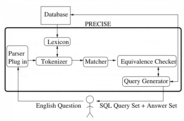
| 23:59, 10 February 2019 | 2003 TowardsaTheoryofNaturalLanguage Fig4.png (file) |  |
57 KB | Omoreira | Figure4: PRECISE System Architecture.In: Popescu et al. (2003). | 1 |
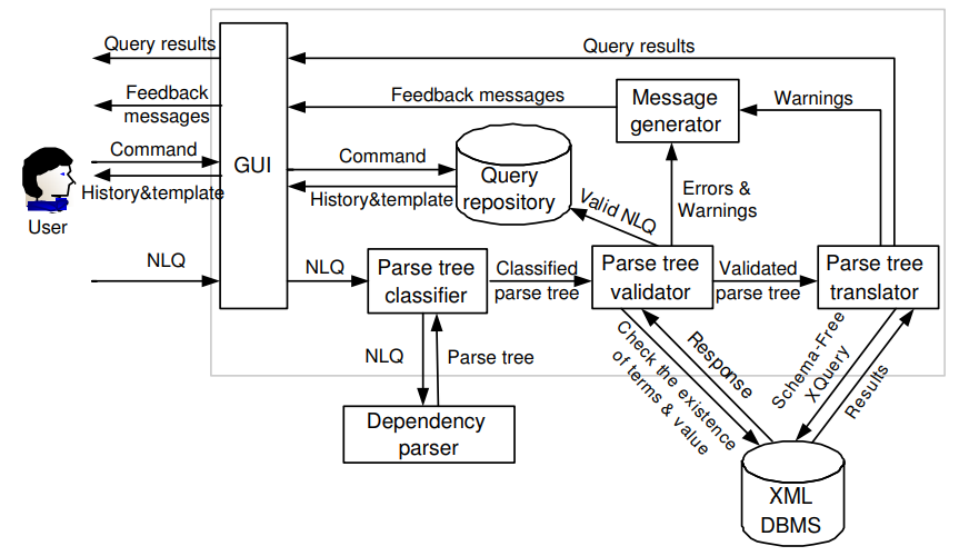
| 23:19, 10 February 2019 | 2005 NaLIXAnInteractiveNaturalLangua Fig1.png (file) |  |
84 KB | Omoreira | Figure 1: Architecture of NaLIX. In: Li et al. (2005). | 1 |
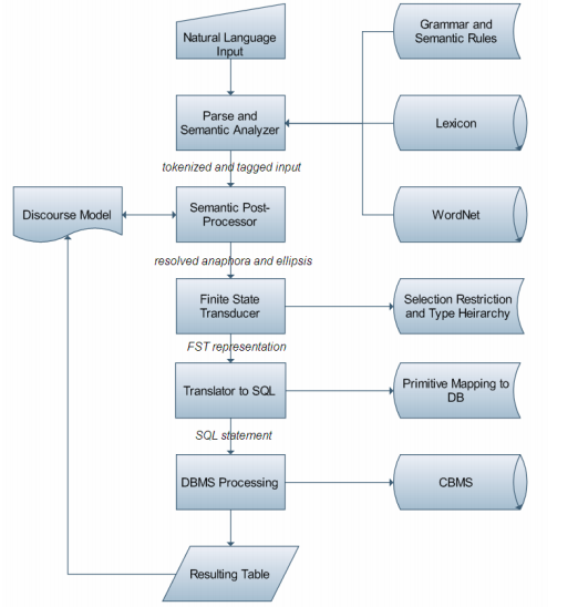
| 08:06, 10 February 2019 | 2008 NaturalLanguageDatabaseInterfac Fig1.png (file) |  |
64 KB | Omoreira | Figure 1: Architectural Design of NLDBI-CBMS. In: Garcia et al. (2008) | 1 |
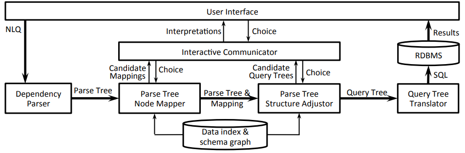
| 06:48, 10 February 2019 | 2014 ConstructingAnInteractiveNatura Fig2.png (file) |  |
42 KB | Omoreira | Figure 2: System Architecture. In: Li & Jagadish (2014). | 1 |
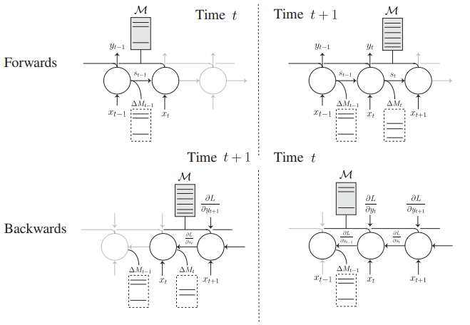
| 23:42, 20 January 2019 | 2016 ScalingMemoryAugmentedNeuralNet Fig5.png (file) |  |
49 KB | Omoreira | Figure 5: A schematic of the memory efficient backpropagation through time. Each circle represents an instance of the SAM core at a given time step. The grey box marks the dense memory. Each core holds a reference to the single [[instan... | 1 |
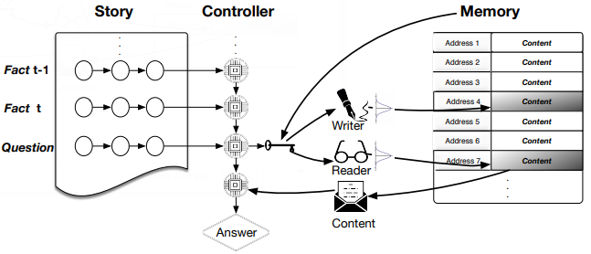
| 20:57, 20 January 2019 | 2016 DynamicNeuralTuringMachinewithS Fig1.png (file) |  |
57 KB | Omoreira | Figure 1: A graphical illustration of the proposed dynamic neural Turing machine with the recurrent-controller. The controller receives the fact as a continuous vector encoded by a recurrent neural network, computes the [[re... | 1 |
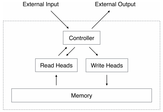
| 23:43, 13 January 2019 | 2014 NeuralTuringMachines Fig1.png (file) |  |
26 KB | Omoreira | '''Figure 1: Neural Turing Machine Architecture.''' During each update cycle, the controller network receives inputs from an external environment and emits outputs in response. It also reads to and writes fr... | 1 |
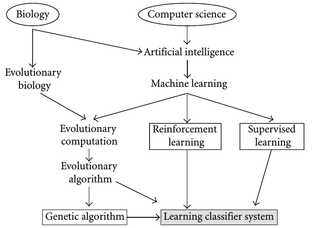
| 07:22, 13 January 2019 | 2009 LearningClassifierSystemsACompl Fig1.png (file) |  |
52 KB | Omoreira | Figure 1: Field tree—foundations of the LCS community. In: Urbanowicz & Moore, (2009) | 1 |
| 14:46, 6 January 2019 | 2018 RethinkingMachineLearningDevelo Fig2.png (file) |  |
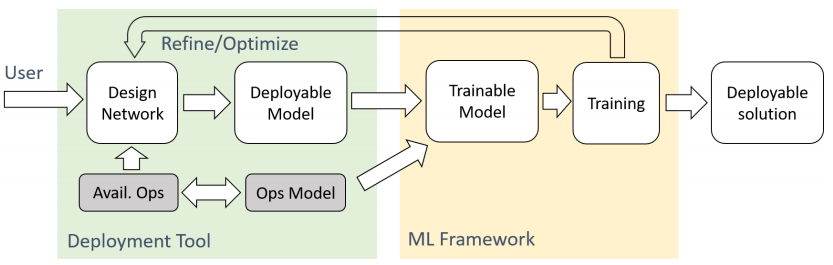
44 KB | Omoreira | <i>Figure 2: Proposed ML development and deployment approach. The shaded blocks are vendor-specific parts</i> In: Lai & Suda, (2018) | 1 |
| 14:41, 6 January 2019 | 2018 RethinkingMachineLearningDevelo Fig1.png (file) | 46 KB | Omoreira | <i>Figure 1: Current ML development and deployment approach. The shaded blocks are vendor-specific parts.</i> In: Lai & Suda, (2018) | 1 | |
| 00:21, 31 December 2018 | 2015 TeachingMachinestoReadandCompre Fig1.png (file) |  |
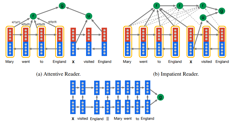
77 KB | Omoreira | Figure 1: Document and query embedding models. In: Hermann et al., (2015). | 1 |
| 23:04, 30 December 2018 | 2016 LSTMbasedDeepLearningModelsforN Fig3.png (file) |  |
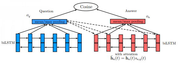
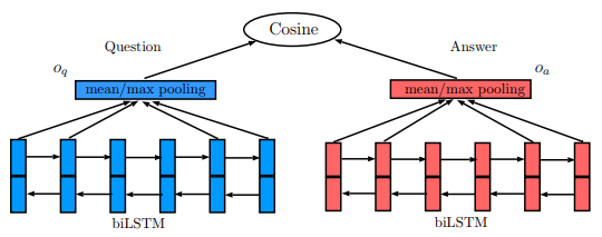
30 KB | Omoreira | Figure 3: QA-LSTM with attention. In: Tan et al., (2016) | 1 |
| 22:46, 30 December 2018 | 2016 LSTMbasedDeepLearningModelsforN Fig2.png (file) |  |
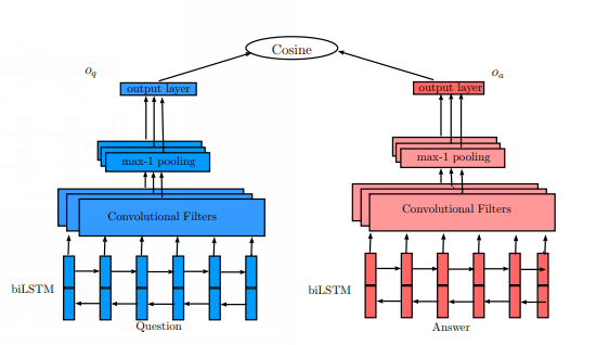
29 KB | Omoreira | Figure 2: QA-LSTM/CNN.In: Tan et al., 2016 | 1 |
| 22:01, 30 December 2018 | 2016 LSTMbasedDeepLearningModelsforN Fig1.png (file) |  |
22 KB | Omoreira | Figure 1: Basic Model: QA-LSTM. In: Tan et al., 2016 | 1 |
| 08:49, 30 December 2018 | 2015 DeepQuestionAnsweringforProtein Fig2.png (file) |  |
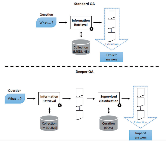
119 KB | Omoreira | Figure 2.</B> Deep QA. In standard QA, answers are extracted from some retrieved documents. In Deep QA, curated data are exploited to build a supervised classification model, which is then used to generate answers. In:[[... | 1 |
| 23:28, 29 December 2018 | 2015 DeepQuestionAnsweringforProtein Fig3.png (file) |  |
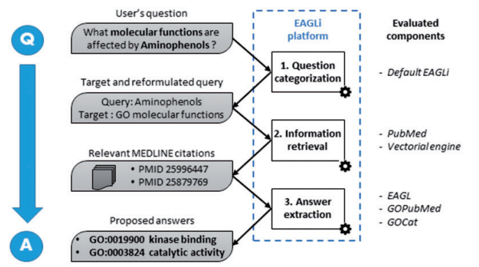
190 KB | Omoreira | <B>Figure 3.</B> Overall workflow of the EAGLi platform. The input is a question formulated in natural language, the output is a set of candidate answers extracted from a set of retrieved MEDLINE abstracts. In: [[2015_De... | 1 |
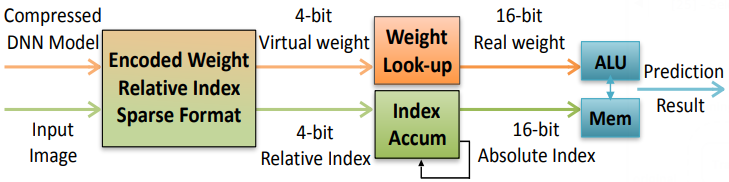
| 17:55, 16 December 2018 | 2016 EIEEfficientInferenceEngineonCo Fig1.png (file) | 48 KB | Omoreira | Figure 1. Efficient inference engine that works on the compressed deep neural network model for machine learning applications. In: Han et al. (2016) | 1 | |
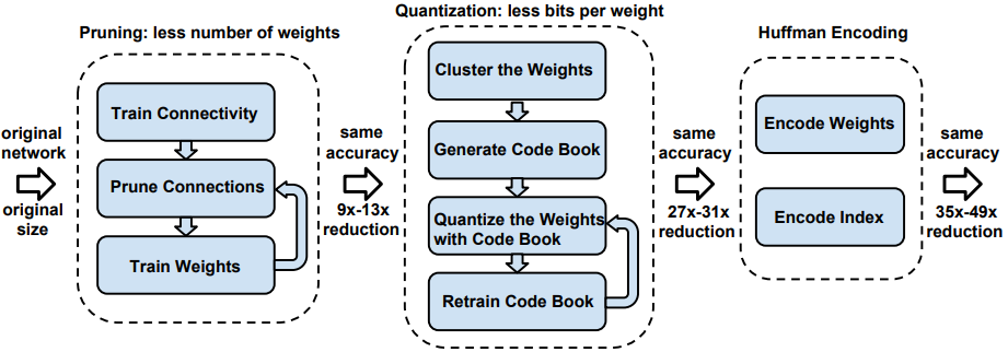
| 16:50, 16 December 2018 | 2016 DeepCompressionCompressingDeepN Fig1.png (file) |  |
74 KB | Omoreira | Figure 1: The three stage compression pipeline: pruning, quantization and Huffman coding. Pruning reduces the number of... | 1 |
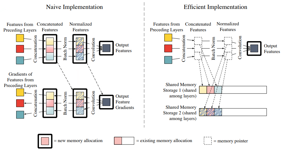
| 11:03, 16 December 2018 | 2017 MemoryEfficientImplementationof Fig3.png (file) |  |
105 KB | Omoreira | Figure 3: DenseNet layer forward pass: original implementation (left) and efficient implementation (right). Solid boxes correspond to tensors all... | 1 |
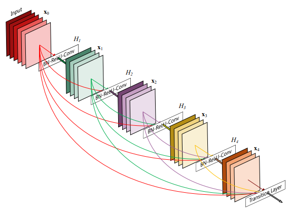
| 10:05, 16 December 2018 | 2017 DenselyConnectedConvolutionalNe Fig1.png (file) |  |
67 KB | Omoreira | Figure 1: A 5-layer dense block with a growth rate of <math>\kappa = 4</math>. Each layer takes all preceding feature-maps as input. In: Huang et al. (2017) | 1 |
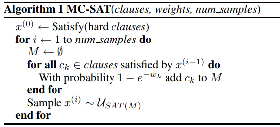
| 16:34, 8 December 2018 | 2006 SoundandEfficientInferencewithP Algorithm1.png (file) |  |
43 KB | Omoreira | Algorihtm 1 ©right; Poon & Domingos, 2006 | 1 |
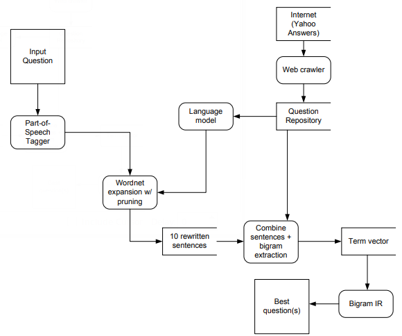
| 00:03, 26 November 2018 | 2018 ProvidingASimpleQuestionAnsweri Fig1.png (file) |  |
32 KB | Omoreira | Figure 1: Overall data flow for our Question ⇒ Question system. In: Larson et al. (2018) | 1 |
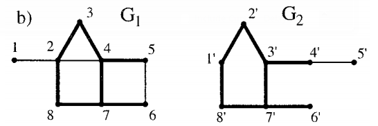
| 08:25, 25 November 2018 | 2002 MaximumCommonSubgraphIsomorphis Fig1b.png (file) |  |
16 KB | Omoreira | <P>Figure 1. b) Maximum common edge subgraph.. In: Raymond & Willett (2002). | 1 |
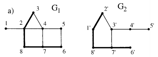
| 08:24, 25 November 2018 | 2002 MaximumCommonSubgraphIsomorphis Fig1a.png (file) |  |
15 KB | Omoreira | <P>Figure 1. a) Maximum common induced subgraph. In: Raymond & Willett (2002). | 1 |
| 07:33, 25 November 2018 | 2002 MaximumCommonSubgraphIsomorphis Fig2b.png (file) |  |
17 KB | Omoreira | Figure 2. b) Disconnected MCES. In: Raymond & Willett (2002) | 1 |
| 07:33, 25 November 2018 | 2002 MaximumCommonSubgraphIsomorphis Fig2a.png (file) |  |
17 KB | Omoreira | Figure 2. a) Connected MCES. In: Raymond & Willett (2002) | 1 |
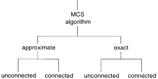
| 04:29, 24 November 2018 | 2002 MaximumCommonSubgraphIsomorphis Fig4.png (file) |  |
16 KB | Omoreira | Figure 4.</B> MCS algorithm classification. In: Raymond & Willett (2002). | 1 |
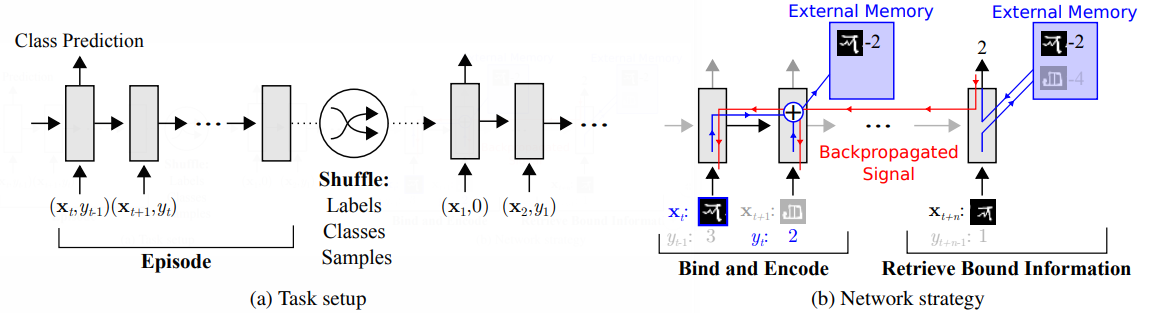
| 23:56, 18 November 2018 | 2016 MetaLearningwithMemoryAugmented Fig1.png (file) | 77 KB | Omoreira | '''Figure 1'''. Task structure. (a) Omniglot images (or x-values for regression), <math>x_t</math>, are presented with time-offset labels (or function values), <math>y_{t−1}</math>, to prevent the network from simp... | 1 | |
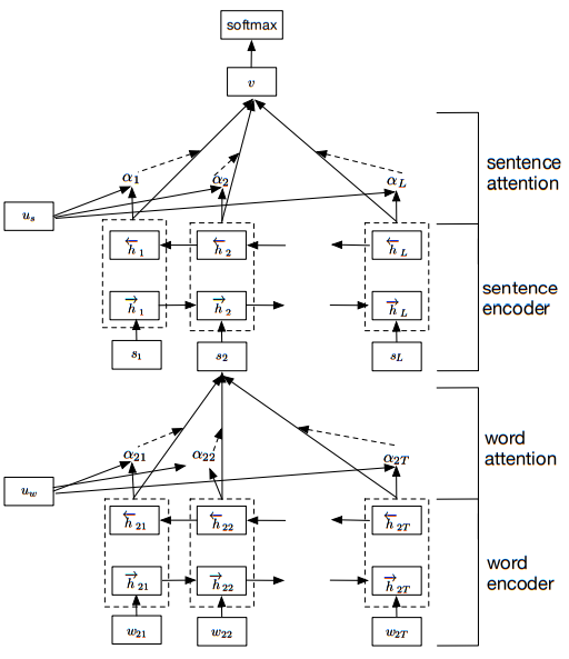
| 22:48, 18 November 2018 | 2016 HierarchicalAttentionNetworksfo Fig2.png (file) |  |
52 KB | Omoreira | '''Figure 2:''' Hierarchical Attention Network. In: Yang et al., (2016) | 1 |
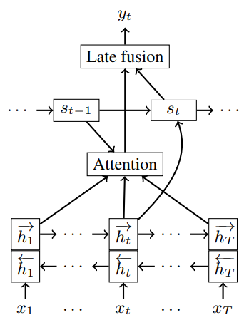
| 05:15, 18 November 2018 | 2016 BidirectionalRecurrentNeuralNet Fig1.png (file) |  |
23 KB | Omoreira | Figure 1: Description of the model predicting punctuation <math>y_t</math> at time step <math>t</math> for the slot before the current input word <math>x_t</math>. In: Tilk & Alumae (2016) | 1 |
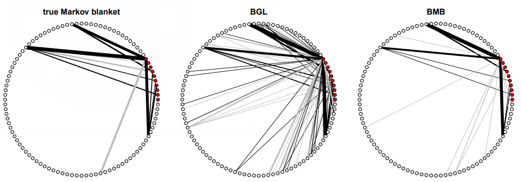
| 06:41, 15 November 2018 | 2015 BayesianMarkovBlanketEstimation Fig2.png (file) | 137 KB | Omoreira | <i><B>Figure 2:</B> One exemplary Markov blanket <math>(p = 10, q = 90)</math> and its reconstruction by BGL and BMB. Note that the graphs only display edges between <math>p</math> query and <math>q</math> remaining variable... | 1 | |
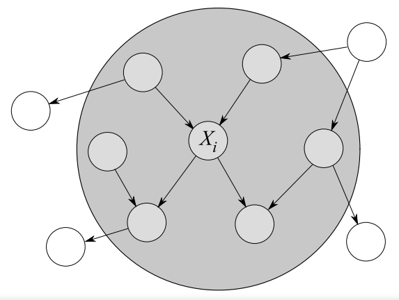
| 06:09, 15 November 2018 | 2006 Kugala Chap4 Fig1.png (file) |  |
40 KB | Omoreira | Figure 4.1: Example of Markov Blanket for node <math>X_i</math>. In: Tomasz Kulaga. (2006).[https://pdfs.semanticscholar.org/cc15/5a644386d8a86ed1124d330e3655e929fe7e.pdf "The Markov Blanket Concept in Bayesian Networks and Dynamic Baye... | 1 |
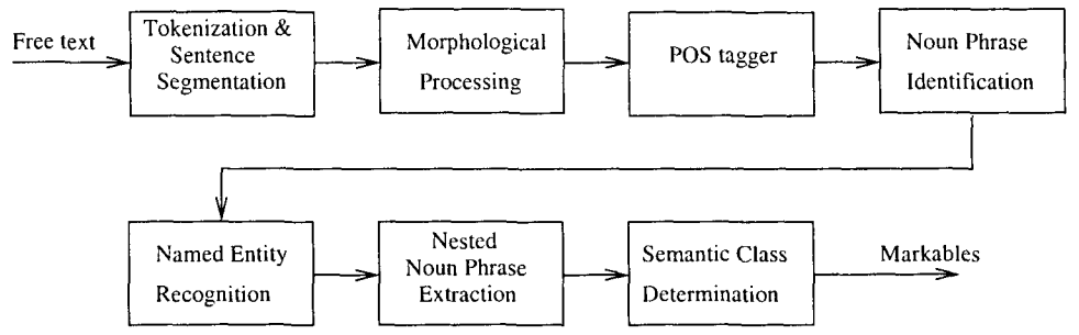
| 22:31, 14 November 2018 | 2001 AMachLearnApprToCorefResOfNounPhrases Fig1.png (file) |  |
48 KB | Omoreira | <B>Figure 1</B> System architecture of natural language processing pipeline. In: Soon et al., (2001) | 1 |
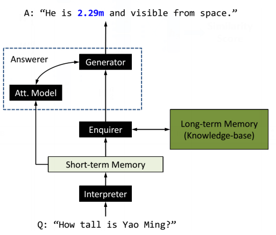
| 19:57, 11 November 2018 | 2016 NeuralGenerativeQuestionAnsweri Fig1.png (file) |  |
50 KB | Omoreira | Figure 1: System diagram of GENQA. In: Yin et al., (2016) | 1 |
| 17:01, 11 November 2018 | 2017 AutomaticQuestionAnsweringUsing Fig4.png (file) |  |
97 KB | Omoreira | '''Fig. 4.''' The block-diagram of the proposed similarity network. IN: Minaee & Liu, 2017 | 1 |
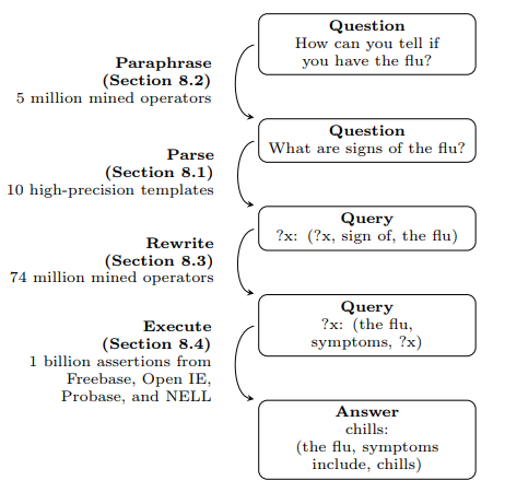
| 23:31, 4 November 2018 | Fader et al 2014 Fig1.png (file) |  |
51 KB | Omoreira | Figure 1: OQA automatically mines millions of operators (left) from unlabeled data, then learns to compose them to answer questions (right) using evidence from multiple knowledge bases. In: Anthony Fader, [[Luke Zet... | 1 |
| 23:51, 28 October 2018 | diags-figure1.png (file) |  |
32 KB | Omoreira | 1 | |
| 23:50, 28 October 2018 | diags-figure0.png (file) | 7 KB | Omoreira | 1 | ||
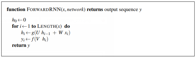
| 23:24, 28 October 2018 | Jurasky Martin 2018 Chap9 Fig5.png (file) |  |
22 KB | Omoreira | <B>Figure 9.5</B> Forward inference in a simple recurrent network. In:Daniel Jurafsky, and James H. Martin (2018). [https://web.stanford.edu/~jurafsky/slp3/9.pdf "Chapter 9 -- Sequence Processing with Recurrent Networks"]. In: [https:/... | 1 |
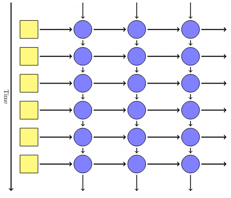
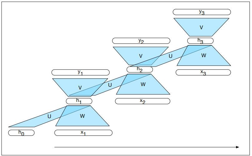
| 23:20, 28 October 2018 | Jurasky Martin 2018 Chap9 Fig4.png (file) |  |
38 KB | Omoreira | <B>Figure 9.4</B> A simple recurrent neural network shown unrolled in time. Network layers are copied for each timestep, while the weights <i>U</i>, <i>V</i> and <i>W</i> are shared in common across all timesteps. In: [[Da... | 1 |
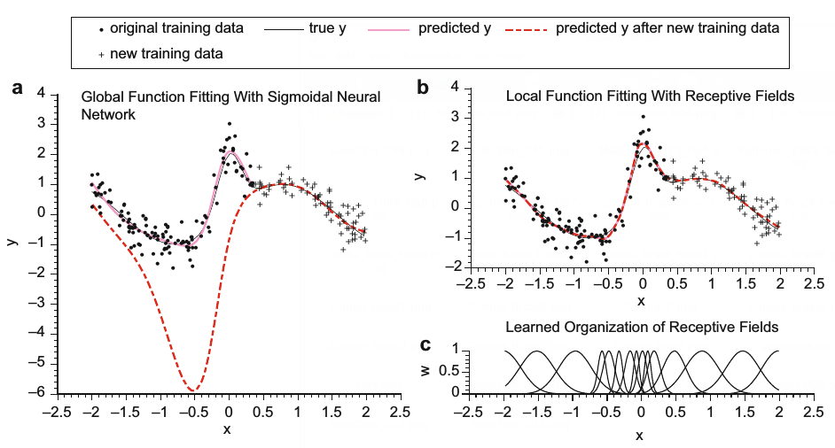
| 15:51, 28 October 2018 | Ting et al 2017 LWRControl Fig1.png (file) |  |
103 KB | Omoreira | .In: Jo-Anne Ting, Franzisk Meier, Sethu Vijayakumar, and Stefan Schaal (2017) [https://link.springer.com/referenceworkentry/10.1007/978-1-4899-7687-1_493 "Locally Weighted Regression for Control"]. In: Sammut & Webb (2017). <P><B>... | 1 |
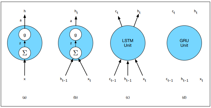
| 20:59, 21 October 2018 | Jurafsky Martin 2018 Chap9 Fig14.png (file) |  |
29 KB | Omoreira | Figure 9.14 Basic neural units used in feed-forward, simple recurrent networks (SRN), long short-term memory (LSTM) and gate recurrent units. In: Daniel Jurafsky, and James H. Martin (2018). [https://web.stanford.edu/~juraf... | 1 |
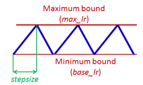
| 04:36, 20 October 2018 | Smith 2017 Fig2.png (file) |  |
37 KB | Omoreira | Figure 2. Triangular learning rate policy. The blue lines represent learning rate values changing between bounds. The input parameter stepsize is the number of iterations in half a cycle. In: Leslie N. Smith (2017, March). [http... | 1 |
| 22:00, 14 October 2018 | D2AG LSTM.png (file) |  |
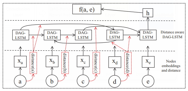
67 KB | Omoreira | Figure 3: D2AG-LSTM In: Zemin Liu, Vincent W. Zheng, Zhou Zhao, Fanwei Zhu, Kevin Chen-Chuan Chang, Minghui Wu, and Jing Ying (2018). [http://forward.cs.illinois.edu/pubs/2017/dagembed-aaai2018-lzzzcwy-201711.pdf "Distan... | 1 |
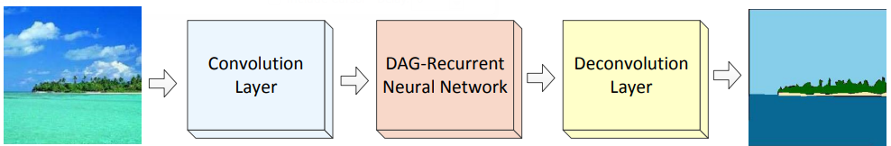
| 21:21, 14 October 2018 | Shuai 1026 DAG RNN Fig3.png (file) | 62 KB | Omoreira | Figure 3: The architecture of the full labeling network, which consists of three functional layers: (1), convolution layer: it produces discriminative feature maps; (2), DAG-RNN: it models the [[conte... | 1 | |
| 20:42, 14 October 2018 | DAG LSTM.png (file) |  |
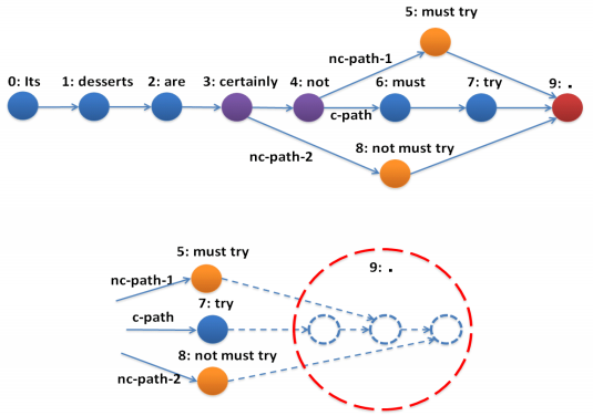
68 KB | Omoreira | Figure 1: An example of DAG-LSTM in modeling a sentence. Nodes with different colors contain different types of LSTM memory blocks. In: Xiaodan Zhu, Parinaz Sobhani, and Hongyu Guo (2016). [http://www.aclweb.org/anthology/N1... | 1 |
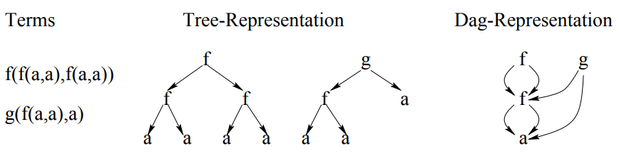
| 17:33, 14 October 2018 | Goller Kuchler 1996 Fig2.png (file) | 22 KB | Omoreira | Figure 2: Tree and DAG representation of a set of terms. In: Christoph Goller, and Andreas Kuchler (1996). [http://citeseerx.ist.psu.edu/viewdoc/download?doi=10.1.1.49.1968&rep=rep1&type=pdf "Learning task-dependent distributed represen... | 1 | |
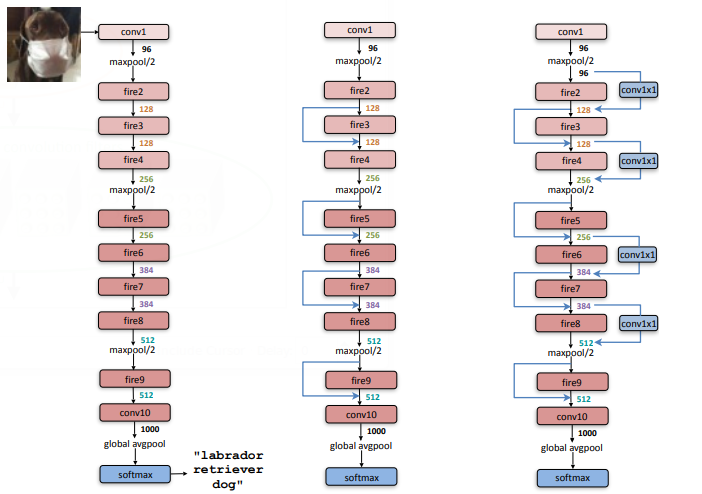
| 23:00, 7 October 2018 | SequeezeNet Architeture.png (file) |  |
86 KB | Omoreira | Figure 2: Macroarchitectural view of our SqueezeNet architecture. Left: SqueezeNet (Section 3.3); Middle: SqueezeNet with simple bypass (Section 6); Right: SqueezeNet with complex bypass (Section 6). In:Forrest N. Iandola, [[Song Ha... | 1 |
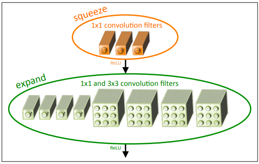
| 23:00, 7 October 2018 | SqueezeNet FireModule.png (file) |  |
56 KB | Omoreira | Figure 1: Microarchitectural view: Organization of convolution filters in the Fire module. In this example, s1x1 = 3, e1x1 = 4, and e3x3 = 4. We illustrate the convolution filters but not the activations. In: Forrest N. Iandola, [[S... | 1 |
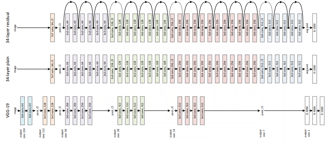
| 23:51, 30 September 2018 | Resnet He 2015 Fig3.png (file) |  |
164 KB | Omoreira | <P>Figure 3. Example network architectures for ImageNet. Left: the VGG-19 model(19.6 billion FLOPs) as a reference. Middle: a plain network with 34 parameter layers (3.6 billion FLOPs). Right: a residual network with 34 parameter layers... | 1 |