2012 ADADELTAAnAdaptiveLearningRateM

where $g_t$ is the gradient of the parameters at the $t$-th iteration $\frac{\partial f(x_t)}{\partial x_t}$ and $\eta$ is a learning rate which controls how large of a step to take in the direction of the negative gradient. Following this negative gradient for each new sample or batch of samples chosen from the dataset gives a local estimate of which direction minimizes the cost and is referred to as stochastic gradient descent (SGD) [1]. While often simple to derive the gradients for each parameter analytically, the gradient descent algorithm requires the learning rate hyperparameter to be chosen.

Setting the learning rate typically involves a tuning procedure in which the highest possible learning rate is chosen by hand. Choosing higher than this rate can cause the system to diverge in terms of the objective function, and choosing this rate too low results in slow learning. Determining a good learning rate becomes more of an art than science for many problems.

This work attempts to alleviate the task of choosing a learning rate by introducing a new dynamic learning rate that is computed on a per-dimension basis using only first order information. This requires a trivial amount of extra computation per iteration over gradient descent. Additionally, while there are some hyper parameters in this method, we has found their selection to not drastically alter the results. The benefits of this approach are as follows:

no manual setting of a learning rate.
insensitive to hyperparameters.
separate dynamic learning rate per-dimension.
minimal computation over gradient descent.
robust to large gradients, noise and architecture choice.
applicable in both local or distributed environments.

2. Related Work

There are many modifications to the gradient descent algorithm. The most powerful such modification is Newton's method which requires second order derivatives of the cost function:

[math]\displaystyle{ \Delta x_{t}=H_{t}^{-1} g_{t} }[/math]

(3)

where $H_{t}^{-1}$ is the inverse of the Hessian matrix of second derivatives computed at iteration $t$. This determines the optimal step size to take for quadratic problems, but unfortunately is prohibitive to compute in practice for large models. Therefore, many additional approaches have been proposed to either improve the use of first order information or to approximate the second order information.

2.1. Learning Rate Annealing

There have been several attempts to use heuristics for estimating a good learning rate at each iteration of gradient descent. These either attempt to speed up learning when suitable or to slow down learning near a local minima. Here we consider the latter.

When gradient descent nears a minima in the cost surface, the parameter values can oscillate back and forth around the minima. One method to prevent this is to slow down the parameter updates by decreasing the learning rate. This can be done manually when the validation accuracy appears to plateau. Alternatively, learning rate schedules have been proposed [1] to automatically anneal the learning rate based on how many epochs through the data have been done. These approaches typically add additional hyperparameters to control how quickly the learning rate decays.

2.2. Per-Dimension First Order Methods

The heuristic annealing procedure discussed above modifies a single global learning rate that applies to all dimensions of the parameters. Since each dimension of the parameter vector can relate to the overall cost in completely different ways, a per-dimension learning rate that can compensate for these differences is often advantageous.

2.2.1. Momentum

One method of speeding up training per-dimension is the momentum method [2]. This is perhaps the simplest extension to SGD that has been successfully used for decades. The main idea behind momentum is to accelerate progress along dimensions in which gradient consistently point in the same direction and to slow progress along dimensions where the sign of the [[gradient] continues to change. This is done by keeping track of past parameter updates with an exponential decay:

[math]\displaystyle{ \Delta x_{t}=\rho \Delta x_{t-1}-\eta g_{t} }[/math]

(4)

where $\rho$ is a constant controlling the decay of the previous parameter updates. This gives a nice intuitive improvement over SGD when optimizing difficult cost surfaces such as a long narrow valley. The gradients along the valley, despite being much smaller than the gradients across the valley, are typically in the same direction and thus the momentum term accumulates to speed up progress. In SGD the progress along the valley would be slow since the gradient magnitude is small and the fixed global learning rate shared by all dimensions cannot speed up progress. Choosing a higher learning rate for SGD may help but the dimension across the valley would then also make larger parameter updates which could lead to oscillations back as forth across the valley. These oscillations are mitigated when using momentum because the sign of the gradient changes and thus the momentum term damps down these updates to slow progress across the valley. Again, this occurs per-dimension and therefore the progress along the valley is unaffected.

2.2.2. ADAGRAD

A recent first order method called ADAGRAD [3] has shown remarkably good results on large scale learning tasks in a distributed environment [4]. This method relies on only first order information but has some properties of second order methods and annealing. The update rule for ADAGRAD is as follows:

[math]\displaystyle{ \Delta x_{t}=-\dfrac{\eta}{\sqrt{\sum_{\tau=1}^{t} g_{\tau}^{2}}} g_{t} }[/math]

(5)

Here the denominator computes the $\ell2$ norm of all previous gradients on a per-dimension basis and $\eta$ is a global learning rate shared by all dimensions. While there is the hand tuned global learning rate, each dimension has its own dynamic rate. Since this dynamic rate grows with the inverse of the gradient magnitudes, large gradients have smaller learning rates and small gradients have large learning rates. This has the nice property, as in second order methods, that the progress along each dimension evens out over time. This is very beneficial for training deep neural networks since the scale of the gradients in each layer is often different by several orders of magnitude, so the optimal learning rate should take that into account. Additionally, this accumulation of gradient in the denominator has the same effects as annealing, reducing the learning rate over time.

Since the magnitudes of gradients are factored out in ADAGRAD, this method can be sensitive to initial conditions of the parameters and the corresponding gradients. If the initial gradients are large, the learning rates will be low for the remainder of training. This can be combatted by increasing the global learning rate, making the ADAGRAD method sensitive to the choice of learning rate. Also, due to the continual accumulation of squared gradients in the denominator, the learning rate will continue to decrease throughout training, eventually decreasing to zero and stopping training completely. We created our ADADELTA method to overcome the sensitivity to the hyperparameter selection as well as to avoid the continual decay of the learning rates.

2.3. Methods Using Second Order Information

Whereas the above methods only utilized gradient and function evaluations in order to optimize the objective, second order methods such as Newton’s method or quasi-Newtons methods make use of the Hessian matrix or approximations to it. While this provides additional curvature information useful for optimization, computing accurate second order information is often expensive.

Since computing the entire Hessian matrix of second derivatives is too computationally expensive for large models, Becker and LecCun [5] proposed a diagonal approximation to the Hessian. This diagonal approximation can be computed with one additional forward and back-propagation through the model, effectively doubling the computation over SGD. Once the diagonal of the Hessian is computed, $\mathrm{diag}(H)$, the update rule becomes:

[math]\displaystyle{ \Delta x_{t}=-\dfrac{1}{\vert \mathrm{diag} \left(H_{t}\right)\vert+\mu} g_{t} }[/math]

(6)

where the absolute value of this diagonal Hessian is used to ensure the negative gradient direction is always followed and $\mu$ is a small constant to improve the conditioning of the Hessian for regions of small curvature.

A recent method by Schaul et al. [6] incorporating the diagonal Hessian with ADAGRAD-like terms has been introduced to alleviate the need for hand specified learning rates. This method uses the following update rule:

[math]\displaystyle{ \Delta x_{t}=-\dfrac{1}{\left|\operatorname{diag}\left(H_{t}\right)\right|} \frac{E\left[g_{t-w: t}\right]^{2}}{E\left[g_{t-w: t}^{2}\right]} g_{t} }[/math]

(7)

where $E\left[g_{t-w: t}\right]$ is the expected value of the previous $w$ gradients and $E\left[g_{t-w: t}^{2}\right]$ is the expected value of squared gradients over the same window $w$. Schaul et al. also introduce a heuristic for this window size $w$ (see [6] for more details).

3. ADADELTA Method

The idea presented in this paper was derived from ADAGRAD [3] in order to improve upon the two main drawbacks of the method: 1) the continual decay of learning rates throughout training, and 2) the need for a manually selected global learning rate.

After deriving our method we noticed several similarities to Schaul et al. [6], which will be compared to below.

In the ADAGRAD method the denominator accumulates the squared gradients from each iteration starting at the beginning of training. Since each term is positive, this accumulated sum continues to grow throughout training, effectively shrinking the learning rate on each dimension. After many iterations, this learning rate will become infinitesimally small.

3.1. Idea 1: Accumulate Over Window

Instead of accumulating the sum of squared gradients over all time, we restricted the window of past gradients that are accumulated to be some fixed size $w$ (instead of size $t$ where $t$ is the current iteration as in ADAGRAD). With this windowed accumulation the denominator of ADAGRAD cannot accumulate to infinity and instead becomes a local estimate using recent gradients. This ensures that learning continues to make progress even after many iterations of updates have been done.

Since storing $w$ previous squared gradients is inefficient, our methods implements this accumulation as an exponentially decaying average of the squared gradients. Assume at time $t$ this running average is $E\left[g^2 \right]_t$ then we compute:

[math]\displaystyle{ E\left[g^{2}\right]_{t}=\rho E\left[g^{2}\right]_{t-1}+(1-\rho) g_{t}^{2} }[/math]

(8)

where $\rho$ is a decay constant similar to that used in the momentum method. Since we require the square root of this quantity in the parameter updates, this effectively becomes the RMS of previous squared gradients up to time $t$:

[math]\displaystyle{ \operatorname{RMS}[g]_{t}=\sqrt{E\left[g^{2}\right]_{t}+\epsilon} }[/math]

(9)

where a constant $\epsilon$ is added to better condition the denominator as in [5]. The resulting parameter update is then:

[math]\displaystyle{ \Delta x_{t}=-\frac{\eta}{\operatorname{RMS}[g]_{t}} g_{t} }[/math]

(10)

3.2. Idea 2: Correct Units with Hessian Approximation

When considering the parameter updates, $\Delta x$, being applied to $x$, the units should match. That is, if the parameter had some hypothetical units, the changes to the parameter should be changes in those units as well. When considering SGD, Momentum, or ADAGRAD, we can see that this is not the case. The units in SGD and Momentum relate to the gradient, not the parameter:

[math]\displaystyle{ \text { units of } \Delta x \propto \text { units of } g \propto \frac{\partial f}{\partial x} \propto \frac{1}{\text { units of } x} }[/math]

(11)

assuming the cost function, $f$, is unitless. ADAGRAD also does not have correct units since the update involves ratios of gradient quantities, hence the update is unitless.

In contrast, second order methods such as Newton's method that use Hessian information or an approximation to the Hessian do have the correct units for the parameter updates:

[math]\displaystyle{ \Delta x \propto H^{-1} g \propto \frac{\frac{\partial f}{\partial x}}{\frac{\partial^{2} f}{\partial x^{2}}} \propto \text { units of } x }[/math]

(12)

Noticing this mismatch of units we considered terms to add to Eqn. 10 in order for the units of the update to match the units of the parameters. Since second order methods are correct, we rearrange Newton's method (assuming a diagonal Hessian) for the inverse of the second derivative to determine the quantities involved:

[math]\displaystyle{ \Delta x=\frac{\frac{\partial f}{\partial x}}{\frac{\partial^{2} f}{\partial x^{2}}} \Rightarrow \frac{1}{\frac{\partial^{2} f}{\partial x^{2}}}=\frac{\Delta x}{\frac{\partial f}{\partial x}} }[/math]

(13)

Since the RMS of the previous gradients is already represented in the denominator in Eqn. 10 we considered a measure of the $\Delta x$ quantity in the numerator. $\Delta x_t$ for the current time step is not known, so we assume the curvature is locally smooth and approximate $\Delta x_t$ by compute the exponentially decaying RMS over a window of size $w$ of previous $\Delta x$ to give the ADADELTA method:

[math]\displaystyle{ \Delta x_{t}=-\frac{\operatorname{RMS}[\Delta x]_{t-1}}{\operatorname{RMS}[g]_{t}} g_{t} }[/math]

(14)

where the same constant $\epsilon$ is added to the numerator RMS as well. This constant serves the purpose both to start off the first iteration where $\Delta x_0 = 0$ and to ensure progress continues to be made even if previous updates become small.

This derivation made the assumption of diagonal curvature so that the second derivatives could easily be rearranged. Furthermore, this is an approximation to the diagonal Hessian using only RMS measures of $g$ and $\Delta x$. This approximation is always positive as in Becker and LeCun [5], ensuring the update direction follows the negative gradient at each step.

In Eqn. 14 the RMS$\left[\Delta x\right]_{t−1}$ quantity lags behind the denominator by 1 time step, due to the recurrence relationship for $\Delta x_t$. An interesting side effect of this is that the system is robust to large sudden gradients which act to increase the denominator, reducing the effective learning rate at the current time step, before the numerator can react.

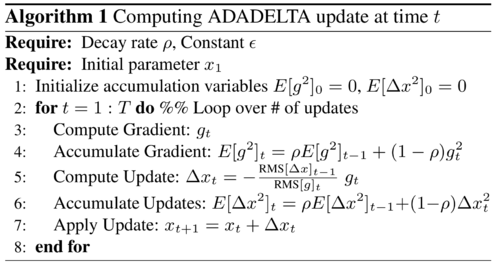
The method in Eqn. 14 uses only first order information and has some properties from each of the discussed methods. The negative gradient direction for the current iteration $−g_t$ is always followed as in SGD. The numerator acts as an acceleration term, accumulating previous gradients over a window of time as in momentum. The denominator is related to ADAGRAD in that the squared gradient information per-dimension helps to even out the progress made in each dimension, but is computed over a window to ensure progress is made later in training. Finally, the method relates to Schaul et al.'s in that some approximation to the Hessian is made, but instead costs only one gradient computation per iteration by leveraging information from past updates. For the complete algorithm details see Algorithm 1.

4. Experiments

We evaluate our method on two tasks using several different neural network architectures. We train the neural networks using SGD, Momentum, ADAGRAD, and ADADELTA in a supervised fashion to minimize the cross entropy objective between the network output and ground truth labels. Comparisons are done both on a local computer and in a distributed compute cluster.

4.1. Handwritten Digit Classification

In our first set of experiments we train a neural network on the MNIST handwritten digit classification task. For comparison with Schaul et al.'s method we trained with tanh nonlinearities and 500 hidden units in the first layer followed by 300 hidden units in the second layer, with the final softmax output layer on top. Our method was trained on mini-batches of 100 images per batch for 6 epochs through the training set. Setting the hyperparameters to $\epsilon = 1e^{− 6}$ and $\rho = 0.95$ we achieve 2.00% test set error compared to the 2.10% of Schaul et al.. While this is nowhere near convergence it gives a sense of how quickly the algorithms can optimize the classification objective.

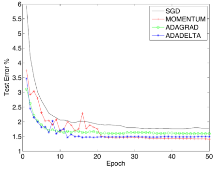
To further analyze various methods to convergence, we train the same neural network with 500 hidden units in the first layer, 300 hidden units in the second layer and rectified linear activation functions in both layers for 50 epochs. We notice that rectified linear units work better in practice than tanh, and their non-saturating nature further tests each of the methods at coping with large variations of activations and gradients.

In Fig. 1 we compare SGD, Momentum, ADAGRAD, and ADADELTA in optimizing the test set errors. The unaltered SGD method does the worst in this case, whereas adding the momentum term to it significantly improves performance. ADAGRAD performs well for the first 10 epochs of training, after which it slows down due to the accumulations in the denominator which continually increase. ADADELTA matches the fast initial convergence of ADAGRAD while continuing to reduce the test error, converging near the best performance which occurs with momentum.

**Fig. 1**. Comparison of learning rate methods on MNIST digit classification for 50 epochs.

4.2. Sensitivity to Hyperparameters

While momentum converged to a better final solution than ADADELTA after many epochs of training, it was very sensitive to the learning rate selection, as was SGD and ADAGRAD. In Table 1 we vary the learning rates for each method and show the test set errors after 6 epochs of training using rectified linear units as the activation function. The optimal settings from each column were used to generate Fig.1. With SGD, Momentum, or ADAGRAD the learning rate needs to be set to the correct order of magnitude, above which the solutions typically diverge and below which the optimization proceeds slowly. We can see that these results are highly variable for each method, compared to ADADELTA in Table 2 in which the two hyperparameters do not significantly alter performance.

**Table 1:** MNIST test error rates after 6 epochs of training for various hyperparameter settings using SGD, MOMENTUM, and ADAGRAD.
	SGD	MOMENTUM	ADAGRAD
$\epsilon = 1e^{0}$	2.26%	89.68%	43.76%
$\epsilon = 1e^{−1}$	2.51%	2.03%	2.82%
$\epsilon = 1e^{−2}$	7.02%	2.68%	1.79%
$\epsilon = 1e^{−3}$	17.01%	6.98%	5.21%
$\epsilon = 1e^{−4}$	58.10%	16.98%	12.59%

**Table 2**: MNIST test error rate after 6 epochs for various hyperparameter settings using ADADELTA.
	$\rho = 0.9$	$\rho = 0.95$	$\rho = 0.99$
$\epsilon = 1e^{−2}$	2.59%	2.58%	2.32%
$\epsilon = 1e^{−4}$	2.05%	1.99%	2.28%
$\epsilon = 1e^{−6}$	1.90%	1.83%	2.05%
$\epsilon = 1e^{−8}$	2.29%	2.13%	2.00%

4.3. Effective Learning Rates

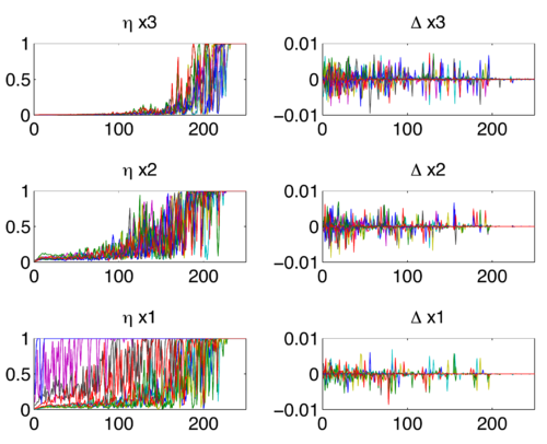
To investigate some of the properties of ADADELTA we plot in Fig.2 the step sizes and parameter updates of 10 randomly selected dimensions in each of the 3 weight matrices throughout training. There are several interesting things evident in this figure. First, the step sizes, or effective learning rates (all terms except gt from Eqn.14 shown in the left portion of the figure are larger for the lower layers of the network and much smaller for the top layer at the beginning of training. This property of ADADELTA helps to balance the fact that lower layers have smaller gradients due to the diminishing gradient problem in neural networks and thus should have larger learning rates.

**Fig. 2**. Step sizes and parameter updates shown every 60 batches during training the MNIST network with tanh nonlinearities for 25 epochs. *Left*: Step sizes for 10 randomly selected dimensions of each of the 3 weight matrices of the network. *Right*: Parameters changes for the same 10 dimensions for each of the 3 weight matrices. Note the large step sizes in lower layers that help compensate for vanishing gradients that occur with backpropagation.

Secondly, near the end of training these step sizes converge to 1. This is typically a high learning rate that would lead to divergence in most methods, however this convergence towards 1 only occurs near the end of training when the gradients and parameter updates are small. In this scenario, the $\epsilon$ constants in the numerator and denominator dominate the past gradients and parameter updates, converging to the learning rate of 1.

This leads to the last interesting property of ADADELTA which is that when the step sizes become 1, the parameter updates (shown on the right of Fig.2) tend towards zero. This occurs smoothly for each of the weight matrices effectively operating as if an annealing schedule was present.

However, having no explicit annealing schedule imposed on the learning rate could be why momentum with the proper hyperparameters outperforms ADADELTA later in training as seen in Fig. 1. With momentum, oscillations that can occur near a minima are smoothed out, whereas with ADADELTA these can accumulate in the numerator. An annealing schedule could possibly be added to the ADADELTA method to counteract this in future work.

4.4. Speech Data

In the next set of experiments we trained a large-scale neural network with 4 hidden layers on several hundred hours of US English data collected using Voice Search, Voice IME, and read data. The network was trained using the distributed system of [4] in which a centralized parameter server accumulates the gradient information reported back from several replicas of the neural network. In our experiments we used either 100 or 200 such replica networks to test the performance of ADADELTA in a highly distributed environment.

The neural network is setup as in [7] where the inputs are 26 frames of audio, each consisting of 40 log-energy filter bank outputs. The outputs of the network were 8,000 senone labels produced from a GMM-HMM system using forced alignment with the input frames. Each hidden layer of the neural network had 2560 hidden units and was trained with either logistic or rectified linear nonlinearities.

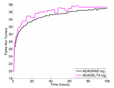
Fig. 3 shows the performance of the ADADELTA method when using 100 network replicas. Notice our method initially converges faster and outperforms ADAGRAD throughout training in terms of frame classification accuracy on the test set. The same settings of $\epsilon = 1e^{−6}$ and $\rho = 0.95$ from the MNIST experiments were used for this setup.

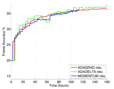
**Fig. 3**. Comparison of ADAGRAD and ADADELTA on the Speech Dataset with 100 replicas using logistic nonlinearities.

When training with rectified linear units and using 200 model replicas we also used the same settings of hyperparameters (see Fig.4). Despite having 200 replicates which inherently introduces significants amount of noise to the gradient accumulations, the ADADELTA method performs well, quickly converging to the same frame accuracy as the other methods.

**Fig. 4**. Comparison of ADAGRAD, Momentum, and ADADELTA on the Speech Dataset with 200 replicas using rectified linear nonlinearities.

5. Conclusion

In this tech report, we introduced a new learning rate method based on only first order information which shows promising result on MNIST and a large scale Speech recognition dataset. This method has trivial computational overhead com pared to SGD while providing a per-dimension learning rate. Despite the wide variation of input data types, number of hidden units, nonlinearities and number of distributed replicas, the hyperparameters did not need to be tuned, showing that ADADELTA is a robust learning rate method that can be applied in a variety of situations.

Acknowledgements

We thank Geoff Hinton, Yoram Singer, Ke Yang, Marc'Aurelio Ranzato and Jeff Dean for the helpful comments and discussions regarding this work.

References

2012a

(Dean et al., 2012) ⇒ J. Dean, G. Corrado, R. Monga, K. Chen, M. Devin, Q. Le, M. Mao, M. Ranzato, A. Senior, P. Tucker, K. Yang, and A. Ng, “Large scale distributed deep networks,” in NIPS, 2012.

2012b

(Jaitly et al., 2012) ⇒ N. Jaitly, P. Nguyen, A. Senior, and V. Vanhoucke, “Application of pretrained deep neural networks to large vo- cabulary speech recognition,” in Interspeech, 2012.

2012c

(Schaul et al., 2012) ⇒ T. Schaul, S. Zhang, and Y. LeCun, “No more pesky learning rates,” arXiv:1206.1106, 2012.

2010

(Duchi et al., 2010) ⇒ J. Duchi, E. Hazan, and Y. Singer, “Adaptive subgradient methods for online leaning and stochastic optimization,” in COLT, 2010.

1988

(Becker & LeCun, 1988) ⇒ S. Becker and Y. LeCun, “Improving the convergence of back-propagation learning with second order methods,” Tech. Rep., Department of Computer Science, University of Toronto, Toronto, ON, Canada, 1988.

1986

(Rumelhart et al., 1986) ⇒ D.E. Rumelhart, G.E. Hinton, and R.J. Williams, “Learning representations by back-propagating errors", Nature, vol. 323, pp. 533-536, 1986.

1951

(Robinds & Monro, 1951) ⇒ H. Robinds and S. Monro, “A stochastic approximation method,” Annals of Mathematical Statistics, vol. 22, pp. 400-407, 1951.

BibTeX

@article{2012_ADADELTAAnAdaptiveLearningRateM,
  author    = {Matthew D. Zeiler},
  title     = {ADADELTA: An Adaptive Learning Rate Method},
  journal   = {eprint arXiv:1212.5701},
  volume    = {abs/1212.5701},
  year      = {2012},
  url       = {http://arxiv.org/abs/1212.5701},
}

	Author	volume	Date Value	title	type	journal	titleUrl	doi	note	year
2012 ADADELTAAnAdaptiveLearningRateM	Matthew D. Zeiler			ADADELTA: An Adaptive Learning Rate Method						2012