2004 FrequentSubtreeMiningAnOverview
- (Chi et al., 2004) ⇒ Yun Chi, Richard R. Muntz, Siegfried Nijssen, and Joost N. Kok. (2001, 2004). "Frequent Subtree Mining - An Overview". In: Fundamenta Informaticae Journal, 66.
Subject Headings: Frequent Tree Pattern; Frequent Subtree Mining Task; Frequent Tree Mining Task.
Notes
Cited By
- Google Scholar:~ 352 Citations (Retrieved:2019-10-06).
- Semantic Scholar: ~ 181 Citations (Retrieved:2019-10-06).
Quotes
Author Keywords
Abstract
Mining frequent subtrees from databases of labeled trees is a new research field that has many practical applications in areas such as computer networks, Web mining, bioinformatics, XML document mining, etc. These applications share a requirement for the more expressive power of labeled trees to capture the complex relations among data entities. Although frequent subtree mining is a more difficult task than frequent itemset mining, most existing frequent subtree mining algorithms borrow techniques from the relatively mature association rule mining area. This paper provides an overview of a broad range of tree mining algorithms. We focus on the common theoretical foundations of the current frequent subtree mining algorithms and their relationship with their counterparts in frequent itemset mining. When comparing the algorithms, we categorize them according to their problem definitions and the techniques employed for solving various subtasks of the subtree mining problem. In addition, we also present a thorough performance study for a representative family of algorithms.
1. Introduction
Data mining, whose goal is to discover useful, previously unknown knowledge from massive data, is expanding rapidly both in theory and in applications. A recent trend in data mining research is to consider more complex cases than are representable by (normalized) single-table relational databases such as XML databases, multi-table relational databases, molecular databases, graph databases, and so on. Databases containing these more complex data types require both practical and theoretical problems to be solved due to the relationships between entities that are thereby introduced.
One of the most general formalisms for modeling complex, structured data is that of the graph. However, graphs in general have undesirable theoretical properties with regard to algorithmic complexity. In terms of complexity theory, currently no efficient algorithms are known to determine if one graph is isomorphic to a subgraph of another. Furthermore, no efficient algorithm is known to perform systematic enumeration of the subgraphs of a given graph, a common facet of a data mining algorithm. One could therefore expect that general graphs pose serious efficiency problems.
Fortunately, many practical databases do not consist of graphs that require exponential computations. The root of the complexity of graph algorithms is often the existence of cycles in the graph. In many cases, the number of cycles in graph instances in a database is limited, or the graphs may even be acyclic. The latter case is especially interesting, e.g., when the graphs are trees, because many very efficient algorithms are known for this Class of graphs. A study of tree mining algorithms may also reveal insights into approaches that can be taken to deal with databases containing graphs instances with few cycles, not only from a practical point of View, but also yielding formal complexity bounds.
In this paper, we review the data mining algorithms that have been introduced in recent years for mining frequent subtrees from databases of labeled trees. We will give an overview of the theoretical properties of these algorithms, and provide the results of experiments in which the tree miners are compared with each other and with a set of frequent graph miners. These results provide a Clearer picture of the most important properties of these algorithms and suggest directions for future research in the field of frequent structure mining.
The importance of graph mining is reflected in the large domain of applications in computer networking, Web mining, bioinformatics, multi—relational data mining, XML document mining, etc. Frequent tree mining algorithms are involved in these applications in many ways:
Gaining general information of data sources When a user faces a new data set, he or she often does not know the Characteristics of the data set. Presenting the frequent substructures of the data set will often help the user to understand the data set and give the user ideas on how to use more specific queries to learn details about the data set. For example, Wang et a1. [42] applied a frequent subtree mining algorithm to a database containing Internet movie descriptions and discovered the common structures present in the movie documentation.
Directly using the discovered frequent substructures Cui et al. [15] showed a potential application of discovering frequent subtrees in network multicast routing. When there are concurrent multicast groups in the network storing routing tables for all the groups independently requires considerable space at each router. One possible strategy is to partition the multicast groups and only build a separate routing table for each partition. Here frequent subtrees among the multicast routing trees of different multicast groups offer hints on how to form the partition.
Constraint based mining Rfickert et a1. [35] showed how additional constraints can be incorporated into a free tree miner for biochemical databases. By extending a free tree miner to mine molecular databases, they found tree shaped molecular fragments that are frequent in active molecules, but infrequent in inactive molecules. These frequently occurring fragments provide Chemists more insight into Quantitative Structure-Activity Relationships (QSARS).
Association rule mining To a commercial online book seller, the information on user patterns of navigation on its web site structure is very important. For example, an association rule that an online book seller may find interesting is “According to the web logs, 90% Visitors to the web page for book A Visited the customer evaluation section, the book description section, and the table of contents of the book (which is a subsection of the book description section).” Such an association rule can provide the book seller with insights that can help improve the web site design.
Classification and clustering Data points in classification and clustering algorithms can be labeled trees. By considering frequent trees as features of data points, the application of standard Classification and clustering algorithms becomes possible. For example, from the web logs of a web site we can obtain the access patterns (access trees) of the Visitors. We might then use the access trees to Classify different types of users (casual vs. serious customers, normal Visitors VS. web crawlers, etc.). As another example, Zaki [50] presented algorithms to Classify XML documents according to their subtree structures.
Helping standard database indexing and access methods design Frequent substructures of a database of labeled trees can provide us with information on how to efficiently build indexing structures for the databases and how to design efficient access methods for different types of queries. For example, Yang et a1. [47] presented algorithms for mining frequent query patterns from the logs of historic queries on an XML document. Answers to the discovered frequent queries can be stored and indexed for future efficient query answering.
Tree mining as a step towards efficient graph mining Nij ssen et a1. [33] have investigated the use of tree mining principles to deal with the more general problem of graph mining. An enhanced tree mining algorithm was shown here to be more efficient than a well—known efficient frequent graph miner.
Recently, many algorithms have been proposed to discover frequent subtrees from databases of labeled trees. These algorithms vary in the specific problem formulations and their solution details. They are, however, similar in many aspects. Most proposed frequent subtree mining algorithms borrow techniques from the area of market—basket association rule mining. In this paper we present an overview of tree mining algorithms that have been introduced until now. Our focus will be on the algorithmic and theoretical differences between these algorithms. We will categorize the algorithms by their problem definitions and the techniques they used to solve various aspects of the subtree mining tasks to expose the common techniques used as well as where they have distinct features.
The rest of this paper is organized as follows. In Section 2, we review necessary theoretical background and terminology. In Section 3, we survey current algorithms for mining frequent subtrees. In Section 4, we discuss other related work. In Section 5, we give a thorough performance study on a representative family of algorithms. Finally, in Section 6, we give future research directions and conclude the paper.
2. Background
In this section we provide necessary background information. We first give an overview of some basic concepts in graph theory, then we discuss different types of labeled trees, and different types of subtrees. Because most frequent tree mining algorithms borrow ideas from frequent itemset mining algorithms, we conclude this section with a review of several types of frequent itemset mining algorithms that have been used effectively in frequent subtree mining.
2.1. Graph Concepts
A labeled graph G 2 (V7 E7 2, L) consists of a vertex set V, an edge set E, an alphabet Z] for vertex and edge labels, and a labeling function L : V U E —) E that assigns labels to vertices and edges. A graph is directed if each edge is an ordered pair of vertices; it is undirected if each edge is an unordered pair of vertices. A path is a list of vertices of the graph such that each pair of neighboring vertices in the list is an edge of the graph. The length of a path is defined by the number of edges in the path. A cycle is a path such that the first and the last vertices of the path are the same. A graph is acyclic if the graph contains no cycle. An undirected graph is connected if there exists at least one path between any pair of vertices, disconnected otherwise.
There are many types of trees. Here we introduce three: unrooted unordered trees (free trees), rooted unordered trees, and rooted ordered trees. In the order listed, the three types of trees have increasing topological structure.
Free tree A free tree is an undirected graph that is connected and acyclic.
Free trees have many properties that can be easily shown; for example, there is a single path between each pair of vertices.
Rooted unordered tree A rooted unordered tree is a directed acyclic graph satisfying (1) there is a distinguished vertex called the root that has no entering edges, (2) every other vertex has exactly one entering edge, and (3) there is a unique path from the root to every other vertex.
In a rooted unordered tree, if vertex v is on the path from the root to vertex w then 1; is an ancestor of w and w is a descendant of v. If, in addition, (1;, w) E E, then 1; is the parent of w and w is a child of v. Vertices that share the same parent are siblings. A vertex that has no descendant other than itself is called a leaf. The depth or level of a vertex is defined as the length of the path from the root to that node.
Rooted ordered tree A rooted ordered tree is a rooted unordered tree that has a predefined ordering among each set of siblings. The order is implied by the left—to-right order in figures illustrating an ordered tree.
So for a rooted ordered tree, we can define the lefi and the right siblings of a vertex, the leftmost and the rightmost child or sibling, etc.
The size of a tree T, denoted as |T|, is defined as the number of vertices the tree has. In this paper, we call a tree of size k a k-tree. A forest is a set of zero or more disjoint trees.
For free trees and rooted unordered trees, we can define isomorphisms between two trees. Two labeled free trees T1 and T2 are isomorphic to each other if there is a one-to-one mapping from the vertices of T1 to the vertices of T2 that preserves vertex labels, edge labels, and adjacency. Isomorphisms for rooted unordered trees are defined similarly except that the mapping should preserve the roots as well. An automorphism is an isomorphism that maps a tree to itself.
As there are different types of trees, there are also different notions of subtrees. Here we give three types of subtrees.
Bottom-up subtree (See [41].) For a rooted tree T (either ordered or unordered) with vertex set V and edge set E, we say that a rooted tree T' (either ordered or unordered, depending on T) with vertex set V' and edge set E' is a bottom-up subtree of T if and only if (1) V’ g V, (2) E' g E, (3) the labeling of V' and E' is preserved in T', (4) for a vertex v E V, if v 6 VI then all descendants of v (if any) must be in V', and (5) if T is ordered, then the left—to-right ordering among the siblings in T should be preserved in T'. Intuitively, a bottom—up subtree T' (with the root 1;) of T can be obtained by taking a vertex v of T together with all v’s descendants and the corresponding edges.
Induced subtree For a tree T (any of the 3 types) with vertex set V and edge set E, we say that a tree T' with vertex set V' and edge set E' is an induced subtree of T if and only if (1) V’ g V, (2) E’ g E, (3) the labeling of V' and E' is preserved in T', (4) if defined for rooted ordered trees, the left—to-right ordering among the siblings in T' should be a subordering of the corresponding vertices in T. Intuitively, an induced subtree T' of T can be obtained by repeatedly removing leaf nodes (or possibly the root node if it has only one Child) in T.
Embedded subtree For a rooted unordered tree T with vertex set V, edge set E, and no labels on the edges, we say that a tree T' with vertex set V', edge set E', and no labels on the edges, is an embedded subtree of T if and only if (1) V’ g V, (2) the labeling of the nodes of V' in T is preserved in T' and (3) (111, 112) E E', where 111 is the parent of v2 in T', only if 111 is an ancestor of 112 in T. If T and T' are rooted ordered trees, then for T' to be an embedded subtree of T, a fourth condition must hold: (4) for 111,112 6 V', preorder(vl) < preorder(v2) in T' if and only if preorder(vl) < preorder(v2) in T, where the preorder of a node is its index in the tree according to the preorder traversal. Intuitively, as an embedded subtree, T' must not break the ancestor- descendant relationship among the vertices of T.
Figure 1 gives examples for the three types of subtrees. In Figure l, for the tree (a) on the left, tree (b) is a bottom—up subtree, tree (C) is an induced subtree but not a bottom—up subtree, tree (d) is an embedded subtree but neither a bottom-up subtree nor an induced subtree. The following relationship among the three types of subtrees follows from the definitions: bottom—up subtree g induced subtrees g embedded subtrees. If T' is a subtree (bottom-up subtree, induced subtree, or embedded subtree) of T, we say T is a supenree of T'.

2.2. Canonical Representations for Labeled Trees
Canonical representations for labeled trees are Closely related to the data structures used to store trees in memory or in disk files. Instead of the standard data structures, such as the adjacency—matrix, the adj acency—list, and the first—child-next—siblin g representation, many tree mining algorithms also use other representations for several reasons. First, some canonical representations are more compact than standard data structures and hence save space. Second, perhaps most importantly, for some types of labeled trees (such as labeled free trees and labeled rooted unordered trees), there can be multiple ways to represent the same tree using the standard data structures. A canonical representation is a unique way to represent a labeled tree. Especially for unordered trees and free trees, the Choice for a canonical representation has far—reaching consequences on the efficiency of the total tree miner. A canonical representation facilitates functions such as comparing two trees for equality and enumeration of subtrees.
In this section we will briefly review various canonical representations for rooted ordered trees, rooted unordered trees, and free trees, respectively. For more detail we refer the reader to the original publications Cited in this section. For simplicity, in the remaining sections, unless otherwise specified, all trees are labeled. In addition, because edge labels can be subsumed without loss of generality by the labels of corresponding nodes (as can be seen shortly, this is true for both rooted trees and free trees), we ignore all edge labels in the following discussion.
String encodings for rooted ordered trees
In [26, 27], Luccio et a1. introduced the following recursive definition for a pre-order string: (1) for a rooted ordered tree T with a single vertex 7', the pre-order string of T is ST = [70, where l, is the label for the single vertex 7', and (2) for a rooted ordered tree T with more than one vertex, assuming the root of T is 7' (with label [7) and the Children of 7' are 7'1, . . . ,rK from left to right, then the pre-order string for T is ST = [,3qu1 --- STTK 0, where ST,1 , . . . , ST, are the pre-order strings for the bottom—up subtrees Tn: . . . ,T,K rooted at 7'1, . . . , rK, respectively. Luccio’s pre—order string for the rooted ordered tree in Figure 1(a) is ST 2 ABDOEOFOOCGOOO. An advantage of Luccio’s pre-order string is that one can easily compute the pre—order string of any bottom—up subtree from the total pre-order string. For example, when we scan ST from label B until we get an equal number of vertex labels and the symbol 0, the resulting substring (BDOEOF 00) is exactly the pre—order string for the bottom-up subtree rooted at B. With such a useful property, the bottom—up subtree matching problem is reduced to the substring matching problem, which can be solved efficiently by algorithms for string matching, e.g., by using the sufix array data structure [17]. It can also be shown that the string encoding is more space-efficient than traditional data structures in storing rooted ordered trees [48].
Similar encodings are also used by Zaki [48] and by Chi et a1. [10, 12]. Asai et a1. [5] and Ni- jssen et a1. [32] independently defined an equivalent encoding for rooted ordered trees using depth sequences. In this encoding the depth of a vertex is explicitly recorded in the string. Again, the pre-order traversal is used. For the tree in Figure 1(a), Asai’s and Nijssen’s string encoding is ST 2 ((0, A), (1, B), (2, D), (2, E), (2, F), (1, C), (2, G)), where each pair represents a vertex: the first num- ber in the pair is the depth of the vertex, and the second symbol is the vertex label. All the string encodings defined by Asai, Nij ssen, and Chi are further extended to canonical representations for rooted unordered trees in the next subsection.
Canonical representations for rooted unordered trees
If one uses standard data structures, such as the adjacency-matrix, the adjacency—list, or the first—child- next—sibling representation, to represent a rooted unordered tree, one faces the following difficulty: because there is no specified order among the children of a vertex, there can be multiple representations for the same tree. The key problem is that from a rooted unordered tree, one can derive multiple rooted ordered trees, as shown in Figure 2.
From these rooted ordered trees we want to uniquely select one as the canonical representation for the corresponding rooted unordered tree. In [26, 27], Luccio et a1. defined such a canonical representation for the rooted unordered tree 7 the sorted pre-order string. The sorted pre-order string for a rooted unordered tree is defined as the lexicographically smallest one among those pre—order strings for the rooted ordered trees that can be obtained from the rooted unordered tree. To determine the lexico- graphical order of the string encodings, a total order on the alphabet of vertex labels is defined. Given a rooted unordered tree, its canonical representation based on the pre-order traversal can be obtained in linear time (assuming a finite alphabet for vertex labels) by adopting Aho’s tree isomorphism algorithm [2], as shown by Luccio et a1. [26, 27]. Later, Asai et a1. [5], Nijssen et a1. [32], and Chi et a1. [10, 11] independently defined similar canonical representations.
Canonical representations for free trees
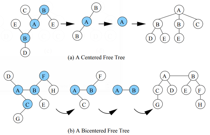
Free trees do not have roots, but we can uniquely define roots for the purpose of constructing a unique canonical representation using the following procedure: starting from a free tree repeatedly remove all leaf vertices (together with their incident edges) until a single vertex or two adjacent vertices remain. For the first case, the free tree is called a centered tree and the remaining vertex is called the center; for the second case, the free tree is called a bicentered tree and the pair of remaining vertices are called the bicenters [3]. A free tree is either centered or bicentered. The above procedure takes linear time. Figure 3 shows a centered free tree and a bicentered free tree as well as the procedure to obtain the corresponding center and bicenters.
Ruckert et a1. [35], Nijssen et a1. [33], and Chi et a1. [10, 12] have shown that if a free tree is centered, one can uniquely identify its center and designate it as the root to obtain a rooted unordered tree, and therefore one can use the canonical representation for the rooted unordered tree to obtain the canonical representation for the centered free tree as was done in the previous section. If a free tree is bicentered, one can cut the free tree into two pieces, each of which is rooted in one of the bicenters, and therefore a canonical string can be obtained by comparing the encodings of the two subtrees. The computation of a canonical string for a free tree consists of two steps: first in linear time the center or the bicenters of the free tree are determined, second the resulting rooted trees are normalized. In total the complexity is therefore also linear.
2.3. Mining Frequent Itemsets
In this section we briefly review the essential parts of frequent itemset mining algorithms. Our purpose is to introduce the concepts that have been exploited in tree mining algorithms by discussing them first in the context of the simpler case of itemset mining.
The problem definition Given an alphabet E of items and a database D of transactions T Q 2, we say that a transaction supports an itemset if the itemset is a subset of the transaction. The number of transactions in the database that support an itemset S is called the frequency of the itemset; the frac- tion of transactions that supports S is called the support of the itemset. Given a threshold minsup, the frequent itemset mining problem is to find the set .7: C 22 of all itemsets S for which support(S) 2 minsup. A well—known property of itemsets, which is the basis of frequent itemset mining algorithms, is that VS' Q S : support(S') 2 support(S). This property is called the a priori property. As an example consider 2 = {A, B, C, D}, D = {{A, B, C}, {A, B, D}, {A, B, C, D}}, and minsup = 2/3, then f = {{A},{B},{0},{D},{A,B}, {A,C},{A,D},{B,C},{B,D},{A,B,C},{A,B,D}}. For itemsets one can easily define a canonical string. The canonical string consists simply of the lexico- graphically sorted list of items: the canonical string for {A, B , D}, for example, is ABD.
Candidate enumeration Given a set of items, all itemsets can be put into a lattice as illustrated in Figure 4. As a consequence of the a priori property of itemsets all frequent itemsets will occupy a connected portion of the lattice, which can be traversed using three alternatives: breadth-first, depth-first, or a combination of the two.
In the breadth-first approach, as shown in Figure 4(a), the search is performed level—wise. First all itemsets of size 1 are generated and counted; then from the frequent l itemsets candidate 2 itemsets are constructed, and so on. If all itemsets are frequent the itemset counting order is: A, B , C, D, AB, AC, AD, BC, BD, CD, ABC, ABD, ACD, BOD, ABCD. In the depth-first approach, as shown in Figure 4(b), the lattice is traversed depth—first. In this case, first itemset A is generated and counted; then, if it is frequent, itemset AB is generated and counted, and so on, resulting in the following evaluation order if all itemsets are frequent: A, AB, ABC, ABCD, ABD, AC, ACD, AD, B, BC, BOD, BD, C, CD, D. The third approach is to use a combination of depth-first and breadth-first traversal, as shown in Figure 4(c). First, all itemsets of size 1 are generated and counted. Then, A is joined with other frequent l-itemsets and the obtained set of 2—itemsets (AB, AC and AD) are recursively investigated further. Only after all itemsets containing item A have been investigated, itemsets which do not contain A are considered. If all itemsets are frequent, the order of itemset counting is: A, B , C, D, AB, AC, AD, ABC, ABD, ABCD, ACD, AD, BC, BD, BOD, CD.
Candidate generation Given a set of k-itemsets, there are several ways to generate an initial set of candidates of size k + 1. One approach is to extend each frequent k-itemset by adding items that are higher (in lexicographic ordering) than the last item in the itemset. For example, given frequent 2- itemsets AB, AC, AD, B C and BD, candidate 3-itemsets formed using extension are ABC and ABD (from AB), AC'D (from A0) and BOD (from B C). When using extension the number of candidates can clearly be very large. This strategy is mostly used in the depth—first traversal of the lattice, in which case it is the only choice for candidate generation. Another candidate generation approach is to join two itemsets. Here each candidate is guaranteed to contain at least two frequent subsets. Most itemset mining algorithms perform the join by joining a pair of k-itemsets that have a common k — 1 prefix. In this approach each itemset has two ancestors in the lattice and less candidates are generated. The breadth- first traversal and the combined depth—first/breadth-first traversal usually adopt join for their candidate generation.
Frequency counting The frequency of a candidate itemset needs to be counted in order to determine if the itemset is frequent. The first frequency counting method is based on direct checking: for each transaction, the frequency of all candidate itemsets supported by the transaction is increased by one. Advanced data structures, such as hash-tree [l], have been used to expedite direct checking. Another frequency counting method is used in vertical mining algorithms [49], which associates an occurrence list (or tid list) with each candidate itemset, i.e., a list of tids of transactions that support it. In such algorithms, the frequency of an itemset is simply the size of the occurrence list. Closely related to vertical mining are the approaches in which the database is re—written into a compact in-memory data structure, where the frequent itemsets together with their frequencies can be extracted from the data structure, without knowing in which transactions the itemsets occur [18].
=== 3. Algorithms for Mining Frequent Subtrees ===
In this section we will systematically study current algorithms for mining frequent subtrees. First, we will formally define the frequent subtree mining problem. For each type of structure we will then study the algorithms in more detail.
3.1. Mining Frequent Subtrees -- The Problem Definition
Given a threshold minfreq, a class of trees C, a transitive subtree relation P j T between trees P, T E C , a finite data set of trees D Q C, the frequent tree mining problem is the problem of finding all trees 73 Q C such that no two trees in ’P are isomorphic and for all P E ’P : freq(P, D) = 21161) d(P, T) 2minfreq, where d is an anti—monotone function such that VT 6 C : d(P', T) 2 d(P, T) if P' j P.
We will always denote a pattern tree 7 a tree which is part of the output 73 7 with a P, and a text tree 7 which is a member of the data set D 7 with a T. The subtree relation P j T defines whether a tree P occurs in a tree T. The simplest choice for function d is given by the indicator function:
In this simple case the frequency of a pattern tree is defined by the number of trees in the data set that contains the pattern tree. We call this frequency definition, which closely matches that of itemset frequency, a transaction basedfrequency. The indicator function is anti—monotone due to the transitiVity of the subtree relation. From the transaction based frequency, one can also easily define a transaction based support: sup(P,D) = freq(P,D)/|D|. Because in some situations a pattern tree may have multiple occurrences in a text tree, other definitions for the frequency of a tree are possible. These are however dependent on the type of tree that is used, and hence we will delay the discussion of other frequency definitions. Unless mentioned otherwise, we assume a transaction based frequency.
In the following discussion, we will use the notation summarized in Table 1.
3.2. Mining Frequent Bottom-Up Subtrees
We first study one of the simplest subtree mining problems: the bottom-up subtree mining problem. From the definition of the bottom-up subtree we can see that the number of bottom-up subtrees for a rooted tree T is the same as the size of T, i.e., the number of vertices T has. (Of course, these bottom-up subtrees might not be all distinct.) As a result, one can solve the frequent bottom-up subtree mining problem in a straightforward way:
1. encode the database in a prefix string format;
2. initialize an array of pointers to each node in the database; note that every pointer points to the root of a bottom-up subtree;
3. sort the pointers by comparing the string encodings of the subtrees to which they point;
4. scan the array to determine the frequencies of the bottom-up subtrees.
| [math]\displaystyle{ t }[/math] | the number of trees in the data set [math]\displaystyle{ D }[/math] |
| [math]\displaystyle{ l }[/math] | the number of distinct labels in data set [math]\displaystyle{ D }[/math] |
| [math]\displaystyle{ m }[/math] | the number of nodes in the largest tree of data set [math]\displaystyle{ D }[/math] |
| [math]\displaystyle{ p }[/math] | the number of nodes in the largest frequent tree |
| [math]\displaystyle{ f }[/math] | the number of frequent pattern trees |
| [math]\displaystyle{ c }[/math] | the number of candidate pattern trees considered by an algorithm |
| [math]\displaystyle{ b = O(pl) }[/math] | the largest number of trees that grow from a single tree |
| [math]\displaystyle{ |V_T| }[/math] | the number of nodes in text tree [math]\displaystyle{ T }[/math] |
| [math]\displaystyle{ |V_P| }[/math] | the number of nodes in pattern tree [math]\displaystyle{ P }[/math] |
| [math]\displaystyle{ |V_D| }[/math] | the number of nodes in database [math]\displaystyle{ D }[/math] |
The key to this straightforward solution is that the number of the bottom-up subtrees for a rooted tree is bounded by |VD|. Also, as shown by Luccio et al. [26, 27], this method applies to both rooted ordered trees and rooted unordered trees, as long as we use the canonical representations for the bottom-up subtrees.
The time complexity of this algorithm is O(m|VD| log |VD|), where m is the size of the largest tree in the database, for the following reasons. Steps 1, 2, and 4 take time O(|VD|). For step 3, the size of the array of pointers is bounded by |VD|. Therefore to use a comparison—based algorithm for sorting, it takes O(|VD| log |VD|) comparisons, where each comparison takes O(m) time because the length of each prefix string is O(m). For rooted unordered trees, we can add a pre—processing step that puts each transaction in the database into its canonical form. As shown by Luccio et a1. [27], the time for canonical ordering of rooted unordered tree with size m is G(m log m) in general, so the pre-processing step takes (m|VD| log m). As a result, the O(m|VD| log |VD|) time complexity applies to rooted unordered trees also. Note that the complexity is independent of the choice for the function d that defines the support.
3.3. Mining Frequent Induced 0r Embedded Subtrees — General Approach
When mining frequent induced or embedded subtrees, the above brute—force method becomes intractable as the number of induced or embedded subtrees for a labeled tree T can grow exponentially with the size of T. (Consider a rooted tree T with |T| — 1 children for the root, all with distinct labels.)
To deal with the potentially exponential number of frequent subtrees, frequent subtree mining algo- rithms for induced subtrees and embedded subtrees usually follow generate-and-test methods. A simple generate-and-test method could be (assume that initially P is an empty tree):
(1) compute freq(P) by determining all T E D 3.75. P j T
(2) let P = succ(P), goto (1).
Here succ(P) is a function which computes the successor of a tree P, such that all possible trees up to maximum size m are enumerated exactly once if one would repeatedly call succ(P).
Of course, this method is not efficient either. Efficient algorithms should at least use the a priori property to restrict the size of the search space. In the next sections we will reveal the details of algorithms that do exactly this. However, from a theoretical standpoint this simple algorithm is still interesting, as in a straightforward way it incorporates two problems that have been studied extensively in the literature:
1. the problem of computing a tree inclusion relation (step (1)).
2. the problem of enumerating all trees in a certain class uniquely (step (2));
Ideally the worst case complexity of subtree mining algorithms should never be higher than that of this naive algorithm. In the next sections, we will use this naive algorithm to set the subtree miners into perspective.
3.4. Rooted Ordered Embedded Subtrees
TreeMiner The TreeMiner algorithm developed by Zaki [48] for mining frequent ordered embedded subtrees follows the combined depth—first/breadth-first traversal idea to discover all frequent embedded subtrees from a database of rooted ordered trees. Other than the general downward closure property (i.e., all subtrees of a frequent tree are frequent), TreeMiner takes advantage of a useful property of the string encodings for rooted ordered trees: removing either one of the last two vertices at the end of the string encoding of a rooted ordered tree P (with correspondent adjustment to the number of backtrack symbols) will result in the string encoding of a valid embedded subtree of P. This is illustrated in Figure 5. If one of the two last vertices in t3, t4, t5 and t6 is removed, either t1 or t2 results. Please note that the removal of the second-to-last vertex of t3 yields tree t2 as we are considering embedded subtrees here. Tree t2 is not an induced subtree of t3, and t3 could not grow from t2 when mining induced subtrees.
From the above discussion it follows that, from a candidate (k+I)-subtree P, we can obtain two of its k-subtrees. One of them, P1, is obtained by removing the last vertex from the string encoding for P; the other, P2, is obtained by removing the second-to—last vertex from the string encoding. In addition, we can see that P1 and P2 share the same (k-I)-prefix (i.e., the string encoding up to the (k-I)-th vertex), and P1 and P share the same k-prefix. It is easier to see the relationship of the (k+I)—subtree to its two k- subtrees, but in the generating of candidate subtrees, the relationship is exploited to generate a candidate (k+I)-subtree through joining two frequent k-subtrees. Because of these properties, TreeMiner is able to follow a combined depth-first/breadth—first traversal where all candidate (k+I)—subtrees are obtained by joining two frequent embedded k-subtrees whose string encodings share the prefix up to the (k-I)—th vertices.
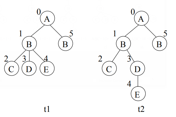
Figure 6 gives a running example of a database consisting of two transactions (with transaction-ids t1 and t2, respectively). For simplicity, we assume the minimum support 3 = 100%. Figure 7 shows the part of the enumeration lattice[1]. that contains all frequent 2-subtrees with A as the prefix and all frequent 3-subtrees with AB as the prefix. From the figure we can see that the candidate generation for TreeMiner is very similar to the combined depth—first/breadth-first lattice traversal of frequent itemset mining.
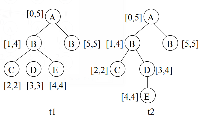
For support counting, TreeMiner uses a method in which the database is rewritten in a vertical repre- sentation of scope lists. For each frequent subtree P with size k, the corresponding scope list records the occurrences of P and, per occurrence, scope information about the last node of P in a pre-order walk, i.e., the so—called rightmost vertex. Each element in the scope list is a triplet (t, M , S )2 t represents the transaction id of the occurrence; M is a list of k-I vertices in the database, to which the first k-I nodes of P (according to a pre-order walk) are mapped; S represents the scope of the rightmost vertex of P . For a vertex v in a text tree T (i.e., a transaction), the scope of v is an interval determined by a pair of numbers. The first number represents the index of 1; according to the pre—order traversal of T, and the second number represents the index of the rightmost child in the bottom-up subtree T(v) induced by 1;. Figure 8 shows the same database as in Figure 6 but with the scope for each vertex given.
Considering a scope as an interval, the scopes S7,1 and S7,2 for two vertices v1 and 112 in the same text tree T are either disjoint intervals (which means that m and v2 have no ancestor-descendant relationship in T), or one interval is a subinterval of the other (which means the vertex with the smaller scope is a descendant of the other vertex in T). Figure 9 shows a join step that uses this scope list data structure. The scope lists of the two frequent 2-subtrees are joined to get the scope list of the resulting candidate 3-subtrees. Elements t and M in the scope list are used to determine if two elements in the scope lists are joinable, and S determines the shape of the resulting candidate subtrees.
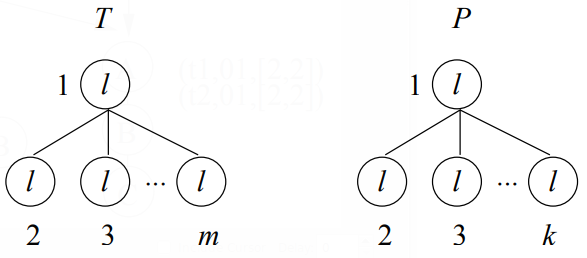
The size of a scope list of TreeMiner may be much larger than the size of a text tree T, as illustrated in Figure 10. The example text tree consists of m vertices connected to a root, while all vertices have the same label; clearly, the number of subtrees of this text tree is small: there are in total m different subtrees. Yet the size of the scope list can be exponential in the size of T: consider the right hand pattern tree P in Figure 10, which consists ofk nodes. There are (72:11) 2 W 2 (7,?7—11)k_1 2 (%)k/2 different subsets of nodes in T to which the nodes of P can be mapped. In a bad case we can assume that p 2 m / 2, so that the support of at least one tree of size k = m / 2 needs to be determined, yielding a list of size 9(2m/4) = 9(29/4) that needs to be constructed. Clearly, the list size is exponential in the worst case. On the other hand, the number of matchings in a tree is always lower than (WM: M210) g ml”. The total size of all scope lists is therefore O(tpmi”) (the additional factor p comes from the size of M in a triplet). If we assume that a list is joined maximally b times, the total work for the construction of scope lists is O( f btpmgi"). The factor 2 in the exponent is due to the quadratic nature of joining embedding lists.
Apart from transaction-based frequencies, rooted tree databases also allow for other frequency definitions, e.g., those based on the root occurrences. If P is isomorphic to a subtree T' of T, then the root of T' (which is a node of T) is called a root occurrence of P in T. If one defines that 7'(P, T) is the total number of root occurrences of P in T, one obtains a function which is also anti-monotone and can be used in a frequency definition. (Please notice that if one uses the frequency that is defined using root occurrences, then one may have support that is greater than 1.) In TreeMiner, a root based frequency can easily be used instead of a transaction based frequency by considering the first element of the matching part M of the scope list triplets.
Complexity Comparison with the Naive Algorithm The enumeration algorithms for embedded subtrees can be implemented in amortized 0(1) time. It was shown in [22] that rooted ordered embedded subtree inclusion can be computed in ®(|VT| |Vp|) time. Therefore for embedded rooted ordered tree mining, the complexity of the naive algorithm can be bounded pessimistically by O(ctpm). Due to the potentially exponential size of TreeMiner occurrence lists, as reflected in the pessimistic upperbound O( f btpmgi”), it is possible that the TreeMiner performs worse than the naive algorithm.
3.5. Rooted Ordered Induced Subtrees
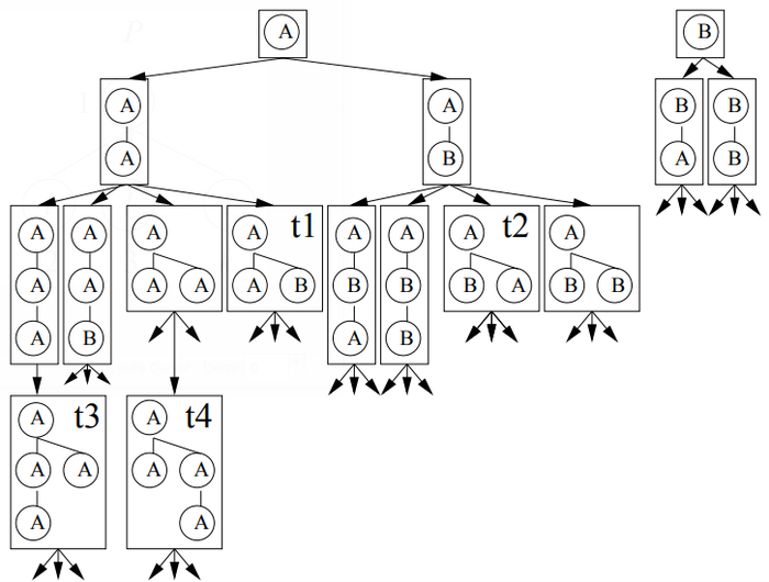
FREQT The FREQT algorithm developed by Asai et al. [4] uses an extension-only approach to find all frequent induced subtrees in a database of one or more rooted ordered trees. In a preprocessing phase, all frequent labels in the database are determined. Then an enumeration tree is built to enumerate all frequent subtrees. To build an enumeration tree, for each (k+I)—subtree Pk+1, one has to identify a unique parent Pk (of size k). In FREQT this problem is solved by removing the rightmost node. If one extends Pk to Pk+1, this means that a new node is connected to the rightmost path of Pk, where the rightmost path is the path from the root of Pk to the last node of Pk in the pre—order. Therefore, in FREQT the set of candidates which are generated from a tree Pk consists of all trees that can be obtained by connecting a new node with a frequent label to the rightmost path. Figure 11 shows a part of the enumeration tree for all rooted subtrees consisting of labels A and B, under the assumption that all possible trees are frequent.
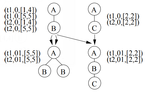
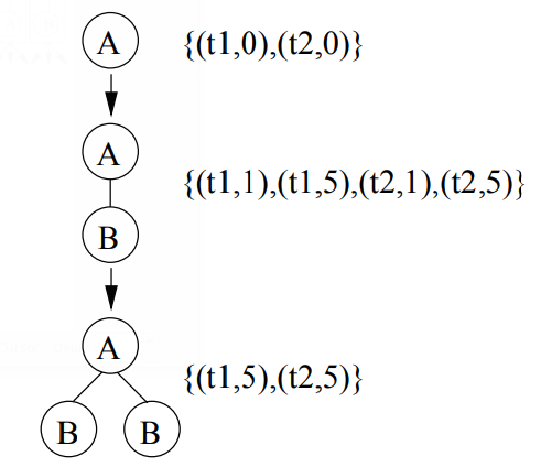
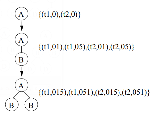
To determine the support of trees FREQT uses an occurrence list based approach. For each subtree, a list records all nodes in the database to which the rightmost node of the subtree can be mapped. Based on the database in Figure 6, a part of the enumeration tree is shown in Figure 12, where the occurrence lists are given. In the example, the occurrence list for the tree PA with a single vertex A is {(t1,0), (t2, 0)}, which means A occurs twice: once in t1 as the 0-th vertex, another time in t2 as the O-th vertex. One extension that is frequent in the example database is PAB (the subtree with two vertices A and B with A being B’s parent). The occurrence list for PAB is {(751, 1), (t1, 5), (t2, 1), (t2, 5)}; here (t1, 1) denotes that the rightmost node of PAB can be mapped to vertex 1 of t1. One can see why for rooted ordered induced subtrees one only has to record the occurrences of the rightmost vertex: only the occurrences of the vertices on the rightmost path are needed for future extension; these occurrences can be derived from the occurrence of the rightmost node. For example, for the tree at the bottom of Figure 12, one only needs to record the occurrences of the rightmost node B , whose occurrence list is {(751, 5), (t2, 5)}. In order to get the occurrence list of the node labeled A, it suffices to scan the occurrence list of the rightmost node B, and to find the parents of the vertices in the occurrence list, which are {(t1,0), (t2, 0)} in our example. Therefore, because the size of occurrence list is bounded by |VD| and is independent of the size of each frequent subtree, the occurrence list method is very scalable when used for support counting of rooted ordered trees.
We now derive a pessimistic upper bound on the time complexity for FREQT. For each frequent subtree T each node v on the rightmost path has to be extended by adding a new rightmost child to v. The size of the occurrence list is bounded by O(|VD|). During the extension of one occurrence at most O(m) nodes in the corresponding text tree are considered, so that a very pessimistic upper bound for FREQT’s time complexity is O(fmIVDD, where f is the number of frequent trees considered. Of course, in real problems the occurrence lists are often much shorter than |VD|.
In FREQT, the number of root occurrences can be easily computed from the occurrence list of the rightmost node. In [4] it was proposed to walk through the database starting from each element in the occurrence list; alternatively one can also add the root occurrence to the occurrence list to avoid a linear recomputation. In addition, although FREQT was developed to mine databases of rooted ordered trees, in special situations it can also be used to mine unordered induced trees. If one assumes that siblings in the database never have the same label, as a preprocessing step one can sort siblings in the database according to their label. All discovered trees will naturally follow the same label order and will reflect the restriction of the database that no two siblings have the same label.
Complexity Comparison with the Naive Algorithm The enumeration algorithm of FREQT can be used by the naive algorithm. The complexity of the enumeration strategy is 0(1) (amortized per enumer- ated tree) and therefore optimal. In [22] it was shown that the complexity of finding all root occurrences of a pattern tree P in a forest D is ®(|Vp||VD|). The total complexity is therefore O(cm|VD|) for the naive algorithm, against O(fm|VD|) for FREQT.
3.6. Rooted Unordered Induced Subtrees
Unot Independently of each other Asai et al. and Nijssen et al. proposed the Unot [5] and uFreqt [32] algorithms, which extend FREQT to mine unordered induced subtrees in the general case that siblings may have the same labels. Candidate generation is conceptually more difficult for unordered trees, as can be seen from the example in Figure 11. While t1 and t2 are different ordered trees, they are isomorphic unordered trees; the same is also true for t3 and t4. Both uFreqt and Unot solve this problem by only enumerating ordered trees with canonical depth sequences. (The canonical depth sequence is equivalent to the pre—order string, as we described in Section 2.2.) That is, among all rightmost path extensions of a subtree in canonical form, only those extensions that result in the canonical form for another subtree are allowed. When a new node is connected to the rightmost path, this corresponds to the concatenation of a new depth tuple at the end of the depth sequence. (Recall that the depth sequence of a rooted unordered tree is a string encoding of the tree which contains both the label and depth for each vertex). It can be shown that the prefix of any canonical depth sequence is itself also a canonical depth sequence, thus the enumeration remains complete if one disregards all extensions that immediately yield a non-canonical sequence.
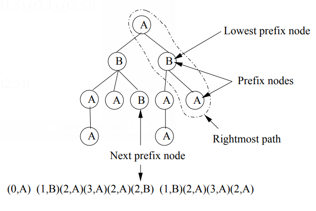
How difficult is it to determine whether an extension is canonical or not? Asai et a1. and Nij ssen et al. use a method which allows for constant time enumeration using depth sequences. We will illustrate the method using the example of Figure 13.
For a rooted unordered tree with a canonical depth sequence, for each node in the tree, we define the depth sequence of that node as the segment of the canonical depth sequence for the tree that corresponds to the bottom-up tree rooted in that node. If a node on the rightmost path has a left sibling in the tree, and its depth sequence is a prefix of the depth sequence of the left sibling, the node on the rightmost path is called a prefix node. The prefix node with the lowest level is the lowest prefix node of the tree. Please note that not every tree has a lowest prefix node. In [5, 32] it was shown that a depth tuple (d, K) may be concatenated after a canonical depth sequence S if and only if:
- if L has a lowest prefix node: d S d', or d = d’ /\ Z 2 Z' must be true, where the next prefix node (d', Z') is obtained as follows. Let i be the length of the depth sequence of the lowest prefix node. Then (d’ , Z') is the (i + 1)th tuple in the depth sequence of the left sibling of the lowest prefix node. In the example, (d', Z') = (2, B); tuples (3, A) and (2, A) may not be concatenated. Intuitively, if one of these tuples would be added, a canonical sequence could be obtained by swapping the order of the children of the root.
- if the rightmost path has a node at depth d with label l', then I 2 l'. In the example, tuple (1, A) cannot be concatenated because A < B.
It was shown in [5, 32] that the index of the next prefix node in the depth sequence can be computed incrementally and in constant time from the index in the unextended depth sequence.
The Unot and uFreqt algorithms differ in the way that the support of trees is evaluated. Unot uses an occurrence list based approach which is similar to that of Zaki’s TreeMiner. For each pattern tree, an occurrence list is constructed which consists of match labels M . Some modifications are introduced to limit the size of the occurrence list. To understand this reconsider the tree at the bottom of Figure 12. In case of unordered induced subtrees for each text tree of Figure 6 there are two possible match labels, 015 and 051, as the two B-labeled vertices can be mapped in two ways to the vertices of the text trees. To avoid that permutations of the same sets of nodes are stored in the occurrence list, in Unot a canonical match label is defined to uniquely pick one out of all possible permutations. For each different set of vertices in the text tree only the canonical match label is stored. By doing this, the worst case list size of Unot is equal to the worst case list size of the TreeMiner, thus exponential. A pessimistic upper bound on the total time complexity for building all occurrence lists is O( f btmp‘l'lp) (see [5] for more details).
uFreqt A different occurrence list based approach was used in the uFreqt algorithm [32]. Here in the worst case for each node in the pattern tree a separate list of occurrences is stored. These lists consist of all the vertices in the data set to which the pattern vertex can be mapped. The size of the occurrence list is therefore bounded by the product of the size of the database and the size of the pattern.
An algorithm is specified that computes new occurrence lists from occurrence lists of the parent tree. This algorithm is shown to be polynomial in the size of the database. In comparison with the simpler matching approach of TreeMiner and Unot, however, the amount of work for each element of the occurrence lists is larger. In [32] it is shown that for each element of the occurrence list, in the worst case a maximum bipartite matching problem has to be solved, for which the worst—case time complexity is O(IVTIV—IVPI)
To determine the extensions of a pattern, the O(| VD|) occurrence list of the rightmost node is scanned; for each element the path to the root in the pattern tree and the neighbors of the occurrences of this path in the text tree are scanned in O(m) time; for each neighbor thus obtained, in the worst case a maximum bipartite matching problem has to be solved for O(p) nodes in the pattern tree to add elements to the occurrence lists of other pattern nodes; the complexity of solving a bipartite matching problem is O(m‘fl—J). The total complexity is therefore 0( f IVDImgp‘fl—J). It should however be noted that a situation in which the size of a list is exactly |VD| and the extension requires m operations, does not exist, and that the upper bound is therefore again very pessimistic.
HybridTreeMiner Chi et a1. [12] proposed an algorithm called HybridTreeMiner that uses the com- bined depth-first/breadth-first traversal approach and generates candidates using both joins and exten- sions. To guarantee that each candidate is generated at most once, HybridTreeMiner uses a canonical form called the breadth—first canonical form, which is based on the level—order traversal. As a conse- quence of this choice, the algorithm cannot determine in constant time which extensions or joins are allowed.
Consider a rooted unordered tree P (in its breadth-first canonical form) with size k + 1. Now, if the last two vertices in the level-order of T are leafs, it was shown in [12] that the breadth-first codes obtained by removing either one of the two last vertices are also canonical, and share a common prefix of size k — 1. However, in the case that the last vertex of the subtree P (in the canonical form) is a child of the second last vertex of P , e.g., trees t3 and t4 in Figure 5, the removal of the second-to-last node would disconnect the tree. Therefore such a tree cannot be obtained from two trees with a common (k — 1) prefix.
These observations can now be used as follows to generate candidates. Given a set of frequent canonical ordered trees of size k that share a common prefix of size (k — 1), each pair of trees in the set is joined; trees which cannot be created through joins are obtained by performing an extension.
As a consequence of the extension, it is necessary to keep the original database also in main memory; it is not possible, as in the TreeMiner, to store the database only in a vertical format. Please notice that here trees are grown by adding leaf nodes from left to right at the lowest level of the tree.
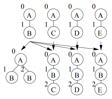
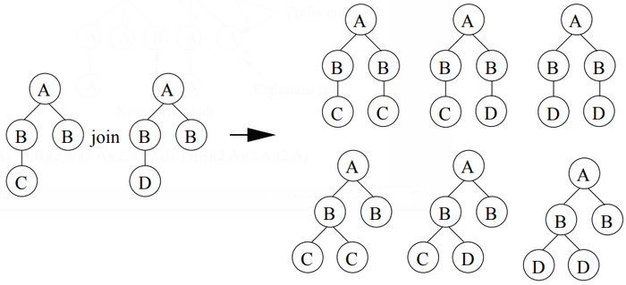
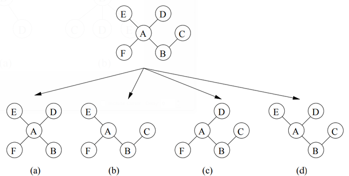
For breadth—first canonical forms an additional problem is that of tree automorphisms when joining two frequent k-subtrees P1 and P2 to obtain a candidate (k+I)—subtree P . Recall that automorphisms of a tree are the isomorphisms of the tree to itself. When joining P1 and P2, if the core (the (k-I)-subtree) shared by P1 and P2 has non-identity automorphisms, the join becomes more complicated. For example, joining (including self—joining) the two trees on the left in Figure 14 results in 6 candidate subtrees. All these 6 candidate subtrees are valid (i.e., they are potentially real frequent subtrees). Chi et al. in [11, 12] provided techniques to store the automorphisms and to use them in the join operation.
Chi et al. show how the occurrence lists of two trees can be joined when a candidate is generated using a join. Because of the join operation, occurrence lists in HybridTreeMiner must record the oc- currences of a candidate subtree in all possible orders, as shown in Figure 15. For example, for the occurrence list of the subtree at the bottom of Figure 15, (t1, 015) and (t1, 051) actually represent the same occurrence in different orders.
The worst case size of the occurrence lists in the HybridTreeMiner can also be computed using the example of Figure 10. In this example there is one possible mapping for the root of P, there are m — 1 nodes to which the first child of the P can be mapped, m — 2 for the second, and so on, for a total of (m— 1)! / (m—k)! occurrences. In general in the worst case there are m!/ (m —p)! 3 m1” possible different occurrences per text tree. If we assume that each occurrence list is scanned during the computation of at most O(b) joins, and one time to find O(m) extensions per occurrence, the total performance is bounded by O(ftm1”(bm1” + m)). Here, the additional factor m1” is again caused by the quadratic nature of joins 7 every occurrence in a list may be joined with multiple elements of another list.
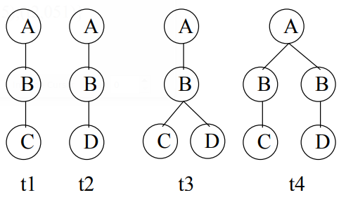
PathJoin Under the assumption that no two siblings are identically labeled, algorithms that mine fre- quent subtrees by joining root paths are feasible. A root path is a path between the root of a tree and a leaf node in the tree. This approach was first taken by Wang et a1. [42] and recently by Xiao et a1. [44] in the PathJoin algorithm. Consider paths t1 and t2 in Figure 16. Although in general the join of these paths is not uniquely defined, if one only allows trees in which siblings have distinct labels, then t3 is the only possible join. Conversely, each unordered tree is defined uniquely by the join of its root paths. The approach which is used in PathJOin [44] is as follows. In a preprocessing step all paths in the database are stored in a FST-Forest data structure. Every root path in the FST—Forest corresponds to a frequent path in the database and has an associated occurrence list. Each element of the occurrence list is a tuple consisting of a tree ID and a node ID; this node ID is the identifier of a node in the database at which the root path starts. We introduce the notation PTg as a short hand for the tree in the FST forest which contains all paths that start with label K. Figure 17 illustrated PTB, based on the database in Figure 6.
If we assume that in a set of siblings of the FST—Forest a label can be found in constant time, the complexity of building the FST—Forest is O(tmg) which follows easily from the observation that all O(mg) paths of all O(t) trees are added iteratively to the FST—Forest.
After the construction of the FST—forest and the determination of all frequent paths, the search for frequent trees starts. We define a r00t-subtree to be an induced subtree of PTg that keeps the root of PTg. A beneficial property of the FST—Forest is that all the frequent subtrees with roots labeled Z are root—subtrees of the tree PTg in the FST—Forest. In our running example, to find all frequent subtrees with root labeled B, we only have to find all the frequent root—subtrees of PTB given in Figure 17. To find all the frequent root—subtrees of a prefix tree PTg, PathJOin uses a variation of the combined depth-first/breadth-first traversal. The search starts with a single node. Then, in a breadth-first fashion all frequent sets of children of the root are determined. Each set of children corresponds to a tree with 2 levels; each such tree is recursively expanded with all possible sets of nodes at level 3, and so on. Overall, all levels are scanned in a depth-first fashion, while all possibilities at each level are determined breadth—first.
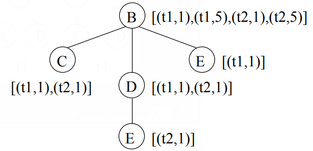
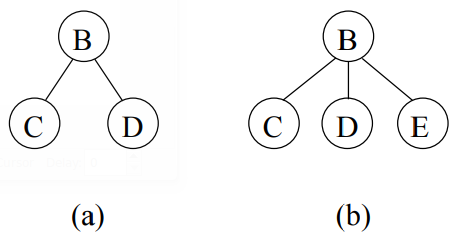
As each pattern tree is a root—subtree of an FST—tree, for each leaf at the lowest level of the pattern tree a potential set of children can be obtained from the FST—tree. The combinations of these candidate children are scanned using a traditional breadth-first algorithm in which two sets of nodes of size k are combined to obtain sets of size k + 1; those candidates which contain an infrequent k subset are removed. The support of each candidate is computed by joining the occurrence lists of all leafs. As an example consider the tree of Figure 18(b). The occurrence list of the path B — C is [(t1,1),(t2,1)]. This list is joined with the occurrence list of path B — D to obtain the occurrence list of the tree in Figure 18(a). This list [(751, 1), (t2, 1)] isjoined with the occurrence list [(751, 1)] of path B — E to obtain the occurrence list [(751, 1)] of the tree in Figure 18(b). Overall, to compute the support of all trees an O(cprpl) computation is required. The total complexity of PathJOin is O(tm2 + cpIVD|).
Complexity Comparison with the Naive Algorithm Because Pathjoin assumes that no two siblings are identically labeled, and because a tree in which all siblings have distinct labels can be mapped to an ordered tree, a problem to which PathJoin applies can also be solved by an ordered tree miner. PathJOin should therefore be compared with the naive algorithm of section 3.5. As O(tm2 + cpIVDI) = O(IVDIm) + O(clepl) = O(chVDD, we may conclude that PathJOin does not introduce a high complexity in the search in comparison with the naive algorithm.
Without the unique sibling assumption, different algorithms are necessary. In [6] an 0(1) algorithm was introduced for enumerating all rooted, unordered trees up to a certain size. Reyner and Matula [34, 29] proposed an algorithm to compute unordered subtree inclusion in O(mp‘fl—J) time. Also this algorithm relies on an algorithm for solving maximal bipartite matching problems. The total complexity of the naive algorithm is therefore O(ctmp‘fl—J). Although the complexity bounds derived for the frequent tree miners are rather pessimistic, still some information can be learned from a comparison of the upper bounds. In uFreqt, with a complexity of O( f IVDImgp‘fl—J), the run time is bounded polynomially. Both Unot and the HybridTreeMiner have an exponential worst case complexity in the size of the largest pattern tree: the complexity of Unot is O(ftmgppbm), where the factor m1” comes from a binomial, while the complexity of the HybridTreeMiner is O( f tm1”(b'm1” + m)), where the factor m1” comes from a factorial. When we compare Unot with the HybridTreeMiner, we see that the number of occurrences in the HybridTreeMiner may be exponentially worse than in Unot, as the HybridTreeMiner does not use a canonical form for match labels. On the other hand, as the HybridTreeMiner uses joins to generate many candidates, in general the branching factor b is smaller in the HybridTreeMiner than in uFreqt, while the number of scans of the data set is also reduced by only considering extensions of the rightmost node.
3.7. Induced Free Subtrees
FreeTreeMiner (1) The FreeTreeMiner algorithm developed by Chi et al. [11] adopts the breadth-first traversal idea to discover all frequent induced subtrees from a database of labeled free trees. The algo- rithm starts with finding all frequent l-subtrees (frequent subtrees with a single vertex), then repeatedly, all candidate (k+I)—subtrees are generated by joining pairs of frequent k-subtrees. For the join operation and the downward closure checking FreeTreeMiner uses the set of leaf vertices, instead of all vertices, of a labeled free tree. Figure 19 gives an example where for downward closure checking for the candidate 6-tree on the top, its leaves are removed one at a time to get all the 5-subtrees (as shown at the bottom of Figure 19) of the 6-tree. For each 5-subtree the canonical string is computed to efficiently search for that subtree in the set of all 5-trees. To meet the downward closure constraint, all the 5-subtrees must be frequent. When generating candidate (k+I)—subtrees, to avoid redundancy, two k-subtrees are joined only if (1) they share a (k-I)-subtree (which is called the core for the pair of k-subtrees), and (2) after joining, the labels of the two leaves other than the core in the two k-subtrees must be the top 2 labels (in the lexicographic order) in the resulting candidate (k+I)—subtree. In the example in Figure 19, although any pair of the 5-subtrees at the bottom can be joined to get the candidate 6—tree on the top, we only join tree (c) and tree (d) because their leaves, other than the core they share, have labels D and E respectively, which are the top 2 leaves in the candidate 6-tree. This method of using the sort order of the leaf labels works fine for trees with distinct vertex labels. When vertex labels are not distinct, the method needs to be changed a little and becomes less efficient [I 1].
To count the support of a candidate subtree P, each transaction T E D is checked to see if P j T. Chung [14] extended the bipartite matching tree inclusion algorithm to subtree isomorphism for free trees, without changing the time complexity. The main idea of Chung’s algorithm is to first fix a root 7' for T (we call the resulting rooted tree T’) then test for each vertex v of P if the rooted tree P” with v as the root is isomorphic to some subtree of T’. Although it may seem that there are more cases to be checked, this is not the case: Chung [14] showed that the time complexity for subtree isomorphisms for free trees is O(|VT||VP| w / |Vp|), which is the same as that for rooted trees. Later, Shamir et a1. improved the time complexity to O(|VT||VP|1/|Vp|/log|Vp|) [36] by solving the maximum bipartite matching problem more efficiently.
One advantage of direct support checking is that no additional information other than the candidate subtrees themselves needs to be stored in memory. This is very important when the number of candidate subtrees is very large and therefore it is impossible to store information other than the candidate subtrees (such as occurrence lists) in memory.
The time complexity of the F reeTreeMiner can be subdivided into two parts: the candidate generation phase and the support counting phase. In the candidate generation phase all frequent trees are combined pairwise to generate new candidates. If we assume that the maximum number of trees generated from one tree is b, at most O(b f / 2) = 0(1) f ) trees are generated. From each of these trees O(p) leafs are removed, the remaining trees are normalized and their existence in the set of frequent trees is checked. Depending on the data structure that is chosen, even in the most efficient data structure this takes O(p) per tree. In total this phase therefore has complexity O(bfpg). To count the frequency of all trees that remain after the frequency based pruning, each of the O(c) candidates is checked in t transactions, making for a worst case complexity of O(ctpfim/ 10g p).
HybridTreeMiner In [12] Chi et al. extend their HybridTreeMiner with breadth-first tree encoding to mine free trees. The HybridTreeMiner is adapted such that only a subset of all rooted trees is considered. More precisely, all trees are disregarded in which the second-deepest subtree of the root is more than one level less deep than the deepest subtree. If one would conceive these special rooted trees as free trees, the special property of these rooted trees is that the root is either the center of the free tree, or one of the bicenters. Thus, by using this simple restriction, the HybridTreeMiner is able to enumerate each centered free tree exactly once, and bicentered free trees at most twice. Using an efficient linear time check, all rooted trees which represent a non-canonical free tree can be removed from the output.
With respect to candidate counting the complexity of this algorithm is similar to that of the Hy- bridTreeMiner for rooted trees: O(ftm7’(bm7’ + m)). Candidate generation is slightly more difficult; to determine whether a candidate is canonical, and to determine automorphisms, a linear algorithm is required.
Gaston Another approach is taken by Nijssen et a1. [33] in the Gaston algorithm. Here the depth- first/breadth-first approach of the HybridTreeMiner is modified to mine free trees using depth sequences. This is achieved by extending a constant time enumeration strategy for unlabeled free trees [31] to labeled trees. As a consequence of this different strategy, it is not necessary to compute the automorphisms of pattern trees to obtain all possible joins. The combined depth-first/breadth-first algorithm uses a procedure which consists of three phases. In the first phase frequent undirected paths are constructed using a combined depth-first/breadth-first approach. During this phase a special canonical form for paths is used which can be computed in linear time. Each of these paths is taken as the starting point of a rooted tree and refined using a subset of rightmost path extensions and joins. In this approach allowable extensions and joins for free trees can be characterized in constant time, while all free trees that are not (almost) a path are enumerated at most once. When the occurrence list based approach of the
HybridTreeMiner is used for frequency evaluation, the complexity of frequency evaluation is the same:
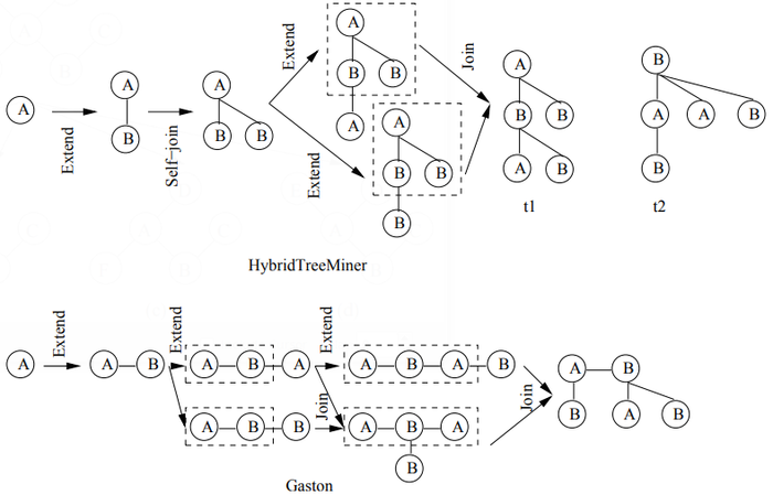
The difference between Gaston and HybridTreeMiner is illustrated in Figure 20. HybridTreeMiner will enumerate both t1 and t2, although they represent the same tree. One can see that in HybridTreeM- iner trees grow level-wise, while in Gaston first paths are grown and trees are constructed from paths. However, the generation of trees from paths in Gaston introduces additional complexity.
FreeTreeMiner (2) In [35] Riickert et al. proposed a FreeTreeMiner which is different from Chi’s FreeTreeMiner [11]. An important difference with the other algorithms is that it searches for frequent free trees in a database of graphs.
Similar to Chi’s FreeTreeMiner, Ruckert’s FreeTreeMiner uses a breadth—first canonical form and grows trees by adding nodes at the lowest level of the tree. The procedure which is used to generate candidates is similar to that of PathJoin. Given a tree with k levels, the algorithm first evaluates its frequency by passing over the database and determining all occurrences of the tree; at the same time, all possible extensions for level k + 1 are determined, together with the transactions that support the extensions. Thus, a set of candidate extensions is obtained. Using a breadth—first approach, instead of frequent subsets, pseudo-frequent subsets of this set of candidates are determined, where the pseudo- frequency is determined by joining the tid lists associated to the candidate extensions. These pseudo- frequencies may be higher than the real frequencies as the locations of the extensions within transactions are not taken into account. For each level thus obtained, the procedure is called recursively to determine the real frequency and find the extensions at the next level.
In our analysis we restrict ourselves to the case that the FreeTreeMiner is applied to a database of trees. As the free tree miner has to determine all possible occurrences of a free tree, the number of occurrences of the free tree that is checked may be O(tmi”); it should be noted here, however, that these occurrences are recomputed each time from scratch. On the one hand, this will increase the computation time (as several matchings will be tried without success before finding good ones). On the other hand, this could reduce the amount of memory used by the algorithm. For each occurrence, the O(m) extensions are determined. Before each tree is really counted, its set of supporting transactions is obtained by computing the intersection of at most O(p) tid lists of size O(t). If we assume that the maximum number of level k + 1 trees obtained from a level k tree is b’ and b is the maximum number of such trees which turn out to have a frequent intersection of tid lists, then a pessimistic upperbound for the total complexity of the FreeTreeMiner is O(f(b'pt + btmp+1)). Complexity Comparison with the Naive Algorithm In [43] an algorithm was given for enumerating unlabeled free trees in 0(1) per enumerated free tree. By defining a bijective mapping between labeled and unlabeled free trees, this algorithm can also be used to enumerate labeled free trees. Using the O(pfim/ log p) free tree inclusion algorithm the inclusion of all 0 trees in the data set can be computed, giving the naive algorithm a worst—case complexity of O(ctpfim/ logp). This closely matches the worst—case complexity of Chi’s FreeTreeMiner, O(ctpfim/ logp). It should be noted however that the candidate generation of Chi’s FreeTreeMiner has much higher complexity than 0(1) per free tree.
All other algorithms have an exponential worst—case complexity: O( f tm1”(b’m;” + m)) for the Hy- bridTreeMiner and Gaston; O( f (b'pt + btmp+1)) for Ruckert’s FreeTreeMiner. The respective advantages or disadvantages of these algorithms are more data set dependent; for example, in comparison with the HybridTreeMiner, Gaston saves the double evaluation of a number of bicentered free trees, but may require the double evaluation of a number of paths.
With respect to the enumeration complexity, there are more differences between the algorithms. Gaston uses an 0(1) strategy for real free trees, and an O(p) scheme for paths. The other algorithms use an O(p) strategy for all structures, where Chi’s FreeTreeMiner and the HybridTreeMiner also require the computation of automorphisms, and Chi’s FreeTreeMiner requires the normalization of free trees for the downward closure test.
4. Other Related Work
Algorithms with inexact matchings Termier et a1. [40] presented an algorithm, TreeFinder, that finds frequent subtrees in a collection of tree-structured XML data (considered as rooted unordered trees). The subtree relationship is defined by tree subsumption. That is, a rooted tree T' is induced according to tree subsumption in another rooted tree T if and only if the ancestor-descendant relationship in T' is a subset of that in T. However, the TreeFinder does not guarantee completeness (i.e., some frequent subtrees may be missed) except for some special cases. Shasha et al. in [37] defined what they called the approximate nearest neighbor search (ANN) problem and presented an algorithm ATreeGrep for searching a query tree in a database of rooted unordered trees. A distance based on approximate containment was used as the tree matching criteria, where the distance between a query tree Q and a text tree D was defined as the total number of Q’s root—to—leaf paths that are not in D. The authors pointed out that although the tree matching is based on root—to—leaf paths, by requiring the distance to be 0 and by using a postprocessing step, the algorithm can be used for exact tree matching.
Maximal and closed frequent subtrees All the algorithms described in this paper discover all frequent subtrees from a database of labeled trees. The number of all frequent induced subtrees and embedded subtrees, however, can grow exponentially with the sizes of the tree-structured transactions. Two con- sequences follow from this exponential growth. First, the end-users will be overwhelmed by the output and have trouble to gain insights from the huge number of frequent subtrees presented to them. Second, mining algorithms may become intractable due to the exponential number of frequent subtrees. The algo- rithms presented by Wang et al. [42] and Xiao et a1. [44] attempt to alleviate the first problem by finding and presenting to end-users only the maximal frequent subtrees. A maximal frequent subtree is a frequent subtree none of whose proper supertrees are frequent. Because they both use postprocessing pruning af- ter discovering all the frequent subtrees, these two algorithms did not solve the second problem. Later, Chi et a1. [13, 9] presented an algorithm, CMTreeMiner, to discover all closed frequent subtrees and maximal frequent subtrees without first discovering all frequent subtrees. A subtree is closed if none of its proper supertrees has the same support as it has. Given a database D and a support 3, the set of all frequent subtrees F, the set of closed frequent subtrees C and the set of maximal frequent subtrees M have the following relationship: M Q C Q .7.
Other types of patterns Other than the three types of subtree relationships (bottom-up, embedded, and induced), there are other types of tree inclusions. In [22], Kilpel'ainen gave a good introduction to many types of tree inclusions in the context of tree matching problems, which includes the definition, applications, and time complexity of each tree matching problem. More recently, Shasha et al. [38] presented an algorithm that discovers all frequent cousin pairs in a single or a set of rooted unordered trees. Two nodes u and v in a rooted unordered tree are a cousin pair if and only if (1) they do not have an ancestor-descendant relationship and (2) if w is the least common ancestor of u and 1;, then the length difference between the path from w to u and that from w to v is either 0 or 1. Shasha et al. showed that mining frequent cousin pairs has many applications such as finding co-occurring patterns in multiple phylogenies, evaluating the quality of consensus trees, and finding kernel trees from groups of phylogenies.
Unlabeled trees In this paper, we focused on databases of labeled trees. Although we can consider unlabeled trees as a special family of labeled trees, the history of research on unlabeled trees is much longer and the theories are much richer than those of labeled trees. For example, according to Asai et a1. [5], Unot directly extended the pattern growth techniques developed first for unlabeled rooted trees by Nakano et a1. [30]. Similarly, Gaston adopted the tree enumeration techniques developed for unlabeled free trees by Nakano et a1. [31]. A comprehensive introduction to the algorithms on unlabeled trees can be found in [41].
Subgraph mining Recently, there have also been studies on mining frequent subgraphs from databases of labeled graphs. Inokuchi et al. [20] presented the AGM breadth-first algorithm for mining frequent unconnected graphs in a graph database. The AcGM algorithm [21] restricts AGM to only find connected subgraphs. Kuramochi et al. [24] presented another breadth-first algorithm for mining frequent subtrees, FSG, which also uses the join operation to generate candidate subgraphs from the frequent subgraphs in the previous level. The AGM algorithm extends subgraphs by adding a vertex per level and the FSG algorithm by adding an edge. The frequent connected subgraph problem was also tackled by Yan et al. [45, 46] in the pure depth-first algorithm gSpan and by Huan et al. [19] in the combined depth- first/breadth-first algorithm FFSM. However, to check if a transaction supports a graph is an instance of the subgraph isomorphism problem which is NP-complete [16]; to check if two graphs are isomorphic (in order to avoid creating a candidate multiple times) is an instance of the graph isomorphism problem which is not known to be in either P or NP-complete [l6].
5. Performance Study
In this section we present a performance study of algorithms for mining frequent embedded subtrees, induced rooted ordered subtrees, frequent induced rooted unordered subtrees, and frequent induced free trees. Table 2 shows the characteristics of all the data sets that we will be using for the performance study and Table 3 gives the explanation for each parameter in Table 2. We will explain each data set in detail in the following discussion.
5.1. Algorithms for Mining Frequent Embedded and Induced Rooted Ordered Subtrees
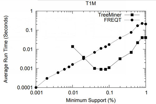
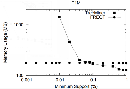
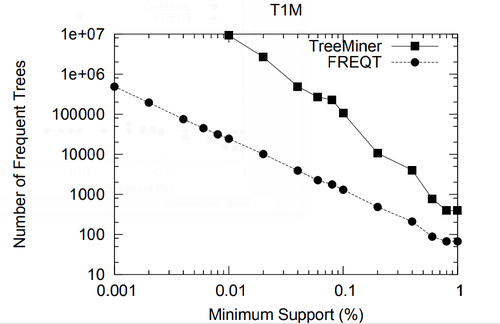
In this section we study the performance of algorithms on mining embedded and induced rooted ordered trees. To the best of our knowledge, at the time of this writing TreeMiner is the only published algorithm for mining the first type of subtrees and FREQT is the only available one for the second type. Therefore, we study the performance of these two algorithms.
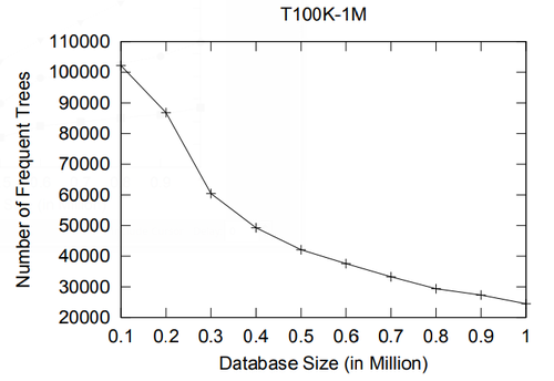
The data set we used is TlM, which is obtained using the generator given by Zaki [48]. This data set mimics web access trees of a web site. We have used the following parameters for the generator: the number of labels N = 100, the number of nodes in the master tree M = 10, 000, the maximum depth D = 10, the maximum fanout F = 10, and the total number of subtrees T = 1, 000, 000.
In the performance study, we mainly use two metrics: the total running time and the memory usage. All experiments in this section and in the next section were done on a 2GHZ Intel Pentium IV PC with 2GB main memory, running the RedHat Linux 7.3 operating system. All algorithms were implemented in C++ and compiled using the g++ 2.96 compiler with -O3 optimization level. For FREQT, we have used Kudo’s implementation given in [23].
Because for a given minimum support, the number of frequent embedded subtrees and the number of frequent induced subtrees are different, we compare the average running time per frequent subtree for TreeMiner and FREQT.
| Name | [math]\displaystyle{ |N| }[/math] | [math]\displaystyle{ |T| }[/math] | [math]\displaystyle{ |N|/|T| }[/math] | [math]\displaystyle{ |F|/|T| }[/math] | [math]\displaystyle{ |max(F)|/|T| }[/math] | [math]\displaystyle{ |D|/|T| }[/math] | [math]\displaystyle{ |N|/|D| }[/math] | [math]\displaystyle{ |L| }[/math] | |||||
| [math]\displaystyle{ \mu }[/math] | [math]\displaystyle{ \sigma }[/math] | [math]\displaystyle{ \mu }[/math] | [math]\displaystyle{ \sigma }[/math] | [math]\displaystyle{ \mu }[/math] | [math]\displaystyle{ \sigma }[/math] | [math]\displaystyle{ \mu }[/math] | [math]\displaystyle{ \sigma }[/math] | [math]\displaystyle{ \mu }[/math] | [math]\displaystyle{ \sigma }[/math] | ||||
| TIM | 2563796 | 1000000 | 2.56 | 2.01 | 1.10 | 0.201 | 1.26 | 0.54 | 2.24 | 1.08 | 1.10 | 0.216 | 100 |
| CS7LOG | 716263 | 59691 | 12.0 | 21.0 | 1.60 | 0.269 | 4.89 | 7.25 | 4.28 | 4.57 | 2.45 | 2.54 | 13209 |
| Multicast | 163753 | 1000 | 163.8 | 62.1 | 1.94 | 0.298 | 5.76 | 1.41 | 257.3 | 1494.8 | 5.83 | 2.16 | 321 |
| T2 (10) | 500000 | 10000 | 50.0 | 0.00 | 1.96 | 0.00 | 6.43 | 1.15 | 11.5 | 1.51 | 4.41 | 0.572 | 1000 |
| D1 | 62936 | 5000 | 12.6 | 13.8 | 1.67 | 0.179 | 5.22 | 4.77 | 3.7 | 1.18 | 3.02 | 2.73 | 10 |
| D2 | 183743 | 10000 | 18.4 | 12.2 | 1.83 | 0.112 | 13.0 | 8.26 | 2.89 | 1.14 | 6.52 | 3.87 | 10 |
| D3 | 62936 | 5000 | 12.6 | 13.8 | 1.67 | 0.179 | 5.22 | 4.77 | 3.7 | 1.18 | 3.02 | 2.73 | 1 |
| [math]\displaystyle{ |N| }[/math] | Number of vertices in the database |
| [math]\displaystyle{ |T| }[/math] | Number of trees in the database |
| [math]\displaystyle{ |N| /|T| }[/math] | Number of vertices per tree |
| [math]\displaystyle{ |F| / |T| }[/math] | Mean fan—out (2 number of adjacent vertices to each vertex) per tree |
| [math]\displaystyle{ |max(F) |/ |T| }[/math] | Maximum fan—out per tree |
| [math]\displaystyle{ |D|/|T| }[/math] | Diameter (= length of longest path in the tree) |
| [math]\displaystyle{ |N|/|D| }[/math] | Number of nodes per tree per diameter (if 1, the tree is a path) |
| [math]\displaystyle{ L }[/math] | Number of labels in the database |
| [math]\displaystyle{ \mu }[/math] | Mean over all trees in the database |
| [math]\displaystyle{ \sigma }[/math] | a Standard deviation over all trees in the database |
From Figure 21(a) we can see that when the minimum support is high, TreeMiner is more efficient. However, as the minimum support decreases, FREQT becomes more efficient while TreeMiner’s average running time increases. A possible reason may be that with a lower value for minimum support, the size of the frequent trees increases. In FREQT the size of a pattern tree does not influence the evaluation time per occurrence; as longer patterns in general have lower support values and therefore fewer occurrences, in FREQT the average computation time per frequent tree decreases. In the TreeMiner, on the other hand, the size of the pattern is of importance as an occurrence contains match labels for all pattern vertices. Combined with possibly longer occurrence lists (due to the exponential nature of the number of occurrences), the amount of computation time in TreeMiner increases with lower minimum support. Figure 21(b) shows the memory usage for the two algorithms under different minimum support (for minimum support less than 0.01%, TreeMiner exhausts all available memory). As we can see from the figure, FREQT’s memory usage remains flat for different minimum support, but TreeMiner increases sharply as the minimum support decreases. The results support our previous observations. For a given minimum support, the total number of frequent embedded subtrees is much larger than that of induced subtrees, as shown in Figure 2l(c). We can see that both the number of frequent embedded subtrees and the number of induced subtrees increase exponentially as the minimum decreases. However, the number of frequent embedded subtrees is much larger (and grows faster) than that of frequent induced subtrees.
5.2. Algorithms for Mining Frequent Induced Rooted Unordered Subtrees
In this section we compare the performance of four algorithms for mining rooted unordered subtrees. They are uFreqt [32], HybridTreeMiner [l2], PathJoin [44], and uFreqt-New, which is an algorithm that combines the enumeration of uFreqt with the occurrence-list based evaluation of the HybridTreeMiner. Because PathJoin does not allow siblings to have the same node labels, experimental results for PathJOin are limited to data sets satisfying this constraint.
CS-LOG The first data set, as described in [48], contains the web access trees of the CS department of the Rensselaer Polytechnic Institute during one month. There are a total of 59,691 transactions and 13,209 unique vertex labels (corresponding to the URLs of the web pages). The average (Zaki’s) string encoding length for the data set is 23.3.
From Figure 22 we can see that the running time for all algorithms remains steady for minimum support greater than 0.3%. After that, as the minimum support decreases further, the running time rises sharply. (Please notice the logarithmic scale of the y-axis.) According to the experiment results, when the minimum support decreases from 0.2% to 0.15%, the number of frequent subtrees grows from 6,855 to 321,437! One possible reason for such an unusual behavior is that as the minimum support falls be- low a certain threshold, the access trees generated by web crawlers, as opposed to regular web surfers, become frequent and these web access trees are usually much larger than the ones generated by regu- lar web surfers. With regard to running time, uFreqt and HybridTreeMiner have similar performance. For memory usage, when the minimum support is lower than 0.3%, uFreqt-New exhausts all available memory. An inspection of the code of both uFreqt-New and the HybridTreeMiner reveals however that the large amount of memory used by both algorithms is partly due to less efficient ways of dealing with large numbers of labels, such as those present in this data set. The HybridTreeMiner has a sharp rise in memory usage at minimum support=0.2%. uFreqt is more scalable in memory usage because of its memory-efficient support counting method.
Multicast The second data set, as described in [13], is a data set of IP multicast trees. The data set consists of MBONE multicast data that was measured during the NASA shuttle launch between the 14th and 21st of February, 1999 [7, 8]. It has 333 distinct vertices where each vertex takes the IP address as its label. The data was sampled from this NASA data set with 10 minutes sampling interval and has 1,000 transactions. This data set is a “dense” one in the sense that there exist strong correlations among transactions. (The transactions are the multicast trees for the same NASA event at different times.) Therefore, frequent subtrees with very large size occur at very high minimum support.
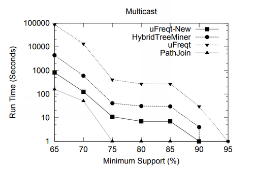
(a)
(b)
(c)
'Figure Figure 23. Performance of Rooted Unordered Tree Miners for the Multicast Data Set.
From Figure 23 we can see that it is difficult for all the algorithms to deal with minimum support values lower than 65%. PathJoin has the best running time performance. However, as the minimum support decreases, the memory usage of PathJoin grows much faster than the other algorithms.
T2 The third data set is generated using the generator given in [13]. In this data set, we want to control the size of the maximal frequent subtrees. A set of |N| (=100) subtrees are sampled from a large base (labeled) graph. We call this set of |N| subtrees the seed trees. Each seed tree is the starting point for |D| - |S| transactions where |D| (=10000) is the number of transactions in the database and |S| (=1%) is the minimum support. Each of these |D| - |S| transactions is obtained by first randomly permuting the seed tree then adding more random vertices to increase the size of the transaction to |T| (=50). After this step, more random transactions with size |T| are added to the database to increase the cardinality of the database to |D|. The number of distinct edge and vertex labels is controlled by the parameter |L| (=10), which is both the number of distinct edge labels and the number of distinct vertex labels. The size of the seed trees |I| ranges from 10 to 30.
The total number of frequent subtrees grows exponentially with the size of the maximal frequent subtrees and thus the running time of the algorithms (other than PathJOin) increases exponentially as well, as shown in Figure 24. In contrast to that of CS-LOG, for this data set the memory usage of the algorithms (other than PathJOin) does not change very much with the number of frequent subtrees (the size of maximal frequent subtrees). This result implies that the memory usage for uFreqt [32], HybridTreeMiner [12] and uFreqt-New depends not only on the number of frequent subtrees, but also on the characteristics of these frequent subtrees. For this data set, uFreqt-New has both the best time performance and the smallest memory usage. PathJoin has very interesting performance for this data set: the running time does not change very much as the size of maximal frequent subtrees grows; however, above a certain size, the memory usage of PathJoin grows and exhausts available memory very quickly. This result, together with the results from other data sets, suggests that the in-memory data structure that used by PathJoin to rewrite the database is proportional to the number of frequent subtrees and therefore may not be scalable in the size of maximal frequent subtrees.
T100K-1M The last data set consists of 10 databases generated using the generator for TlM [48]. All parameters remained the same as those in TlM, except that the number of transactions in each database grows from 100,000 to 1, 000, 000. This data set is designed to test the scalability of the algorithms with respect to the database size.
As shown in Figure 25, with a fixed minimum support (0.01%), as the database size increases, both the running time and the memory usage grow linearly. The running time of uFreqt grows much faster than that of the other algorithms, although the growth is sublinear for the databases under study. Therefore, according to this study, all three algorithms, uFreqt [32], HybridTreeMiner [12] and uFreqt-New, have good scalability with respect to the database size. It is interesting to notice that as the database size increases, for the same minimum support, the total number of frequent subtrees decreases exponentially. This is mainly due to the way that the data set generator is implemented.
Conclusions Among the algorithms on mining frequent rooted unordered subtrees, for most of the data sets that we have studied, uFreqt-New has the best time performance (except for Multicast) and the smallest memory footprint (except for CS-LOG). For the Multicast data set, PathJoin has the best time performance; for the CS-LOG data set, uFreqt has the smallest memory usage. All the algorithms have good scalability in the database size. However, our study suggested that the memory usage of PathJOin was directly affected by the total number of frequent subtrees. In addition, by comparing the CS-LOG data set and the T2 data set, we can see that the memory usage of the other algorithms depends not only on the total number of frequent subtrees, but also on other parameters, such as the size of the patterns.
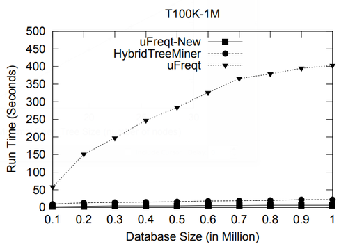
(a)
(b)
(c)
'Figure 25. Performance of Rooted Unordered Tree Miners for the TlOOK—lM Data Set (minsup = 0.01%)]]
5.3. Algorithms for Mining Frequent Induced Free Trees
In this section we study the performance of several free tree mining algorithms discussed in this pa- per: the HybridTreeMiner [12], the FreeTreeMiner [11] and Gaston [33][2]. As free tree databases are graph databases, we also include graph mining algorithms in our experimental results; more precisely, we consider the breadth-first graph miners FSG [24] and AcGM [21], and the depth—first graph miner gSpan [45]. Here we also use two metrics: the total running time and the memory usage. Except when stated otherwise, experiments were done on a 2.8GHz Intel Pentium IV PC with 512MB main memory, running the RedHat Linux 7.3 operating system. All algorithms were implemented in C++. All free tree mining algorithms were compiled using the g++ 2.96 compiler with -O3 optimization level. Of the graph miners we obtained binaries which were compiled under similar circumstances, except for AcGM, which was compiled using a more recent compiler. We will report on an experiment with AcGM for an AMD Athlon XP1600+ with 512MB main memory, running the Mandrake Linux 9.1 operating system.
CS-LOG In this experiment, we use the same CS-LOG data set that was also used in the previous section when mining rooted trees. Clearly, it can also be interesting to know the browsing behavior when the point of entry is not taken into account. The gSpan algorithm is not considered in this experiment as the binary module made available did not allow for more than 255 labels. Our experimental results as reported in Figure 26 (nextpage)revea1 similar characteristics as we found in our experiments for rooted trees: below a certain threshold, the number of frequent trees explodes. The HybridTreeMiner and Gaston run out of memory below this threshold as the sizes of the embedding lists of these algorithms increase dramatically. The breadth—first miners do not suffer from this memory exhaustion problem, but still the computation time for the F reeTreeMiner increases drastically. The breadth-first FSG graph miner requires less memory and manages to scale better with smaller thresholds. We will consider possible explanations for this phenomenon when discussing experimental results on artificial data sets in the next paragraph.
Artificial Data Sets D1, D2 and D3 In this section we use several artificial data sets that were generated by a modified generator as described in [48]. In the modification, we pose constraints on the minimum and maximum size of the trees that are generated; furthermore, we allowed for a stricter control of the fanout of trees that are generated. The parameters of the data sets are summarized in Table 2.
Data set D1 is a small data set and has a low fanout, while the number of labels is rather high. Such characteristics reflect the properties of application domains in web-browsing and molecular mining. This experiment therefore gives a reasonable indication of the performance of the free tree miners on many practical, but not too large databases. As reflected in Figure 27(a), the depth-first mining algorithms perform better here than the breadth-first miners.
In Figure 27(b) one sees that the amount of memory for relatively low support values increases for both the breadth-first and depth-first mining algorithms, with the exception of gSpan. The breadth-first mining algorithms require a large amount of memory to store all candidates in main memory, while the occurrence list based tree miners require memory for storing the occurrence lists. gSpan performs better memory-wise as it only stores the identifiers of trees in which a pattern graph occurs, and not the occurrences itself.
Figure 27(c) shows the effect of increasing data set size. Due to the large differences in run times, we had to show this graph in a logarithmic scale. All algorithms scale linearly in the size of the database. The scale-up properties of FSG suggest that this algorithm includes additional features to deal with many similar graphs in the input.
In data set D2 we specified a very large fanout in combination with a relatively low number of labels. This is reflected in Table 2 by high mean value for |N| / |D|. A value of 1 would indicate that a tree is a path. The resulting trees are rather broad and not very deep; in this way we obtain data sets which exhibit the bad case situation of Figure 10.
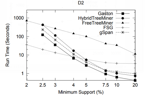
(a)
(b)
(c)
Figure 28. Performance of Free Tree Miners and Graph Miners for the D2 and D3 Data Sets]]
In Figure 28(a) we can see that the depth-first miners are now no longer advantageous in compar- ison with the breadth-first miners. For low values of minimum support, the runtime for the depth-first algorithms increases much more than that of the breadth—first tree miners. The reason for this behav- ior becomes clear when one considers the memory usage of the algorithms. The memory usage of the full occurrence based tree miners rises exponentially for low values of support, which indicates that the number of different occurrences of some lower frequent trees is very large. This behavior can partly be explained when one considers the large fan—out of this data set in combination with the low number of labels. It is very likely that several siblings have the same label and that frequent trees have many symmetries. All depth-first algorithms use an extension-based approach which means that in order to extend a pattern tree, they have to consider all occurrences of a pattern tree in the text tree in order to find all possible extensions. For this particular database this amounts to a large number of possibilities, all of which are stored in the occurrence based algorithms, and all of which have to be considered by the depth-first algorithms. The breadth-first algorithms prune the search space better.
This situation is stressed even further in data set D3 (see Figure 28(c)), which is equal to data set D1, except that all labels have been removed. Without labels the number of occurrences rises rapidly and all occurrence-list based algorithms run out of memory almost immediately, even though the data set is not extremely large. An exception to this rule is gSpan: as gSpan does not store occurrence lists, but recomputes all occurrences, the applicability of gSpan is not limited by the amount of main memory; gSpan however clearly also shows the extremely large run times which can be expected from algorithms that have to check all occurrences.
Another interesting conclusion can be drawn from the comparison of the FreeTreeMiner and FSG on data set D3. Although in all other experiments FSG performs better than the FreeTreeMiner, the situation is completely different when the labels are left out of the data set. In this case, it appears that the polynomial tree inclusion algorithm of the FreeTreeMiner performs better than the potentially exponential subgraph isomorphism algorithm of FSG. This also provides an explanation for the overall good performance of the graph miners: as long as there is a reasonable number of labels, the subgraph isomorphism problem is in practice efficiently solved.
6. Conclusion and Future Directions
The aim of this paper has been to examine the current algorithms for mining frequent subtrees from databases of labeled trees. We started by giving applications of frequent tree mining algorithms. Then we introduced relevant theoretical background in graph theory and we studied some representative a1- gorithms in detail. We have focused our study on two main components of these algorithms 7 the candidate generation step and the support counting step. Next we presented thorough performance studies on a representative family of algorithms. We also discussed some related work such as approximate algorithms and algorithms for mining closed and maximal frequent subtrees.
Regarding efficiency issues, our performance study revealed that there is no single best tree mining algorithm. Some algorithms offer a better time efficiency, while other algorithms require less memory. With respect to the free tree mining algorithms, we may conclude that the performance of current free tree miners does not differ very much from that of the more general graph mining algorithms. There may be several reasons for this:
- although in general subgraph isomorphism is NP complete, in common cases the required compu- tations are not exponential at all. For example consider the case that all labels in a pattern and a text graph (see Section 3.1) are different: subgraph isomorphism can then be checked very efficiently by checking the edges between equally labeled nodes in both graphs. Most graph miners use very label oriented approaches which are very well suited for such situations. In practice, therefore, graph miners can compute subgraph isomorphism and graph isomorphism also very efficiently, although for different reasons than the frequent tree miners.
- although subtree inclusion is computable polynomially, all current occurrence—list based free tree miners do not take advantage of this property and use potentially exponential occurrence lists; in [33] it was even shown that the occurrence lists used by tree miners are straightforwardly expanded to the more general graph mining case.
- the implementations of some graph miners are much older than those of the tree miners and have been repeatedly optimized in recent years [24, 25]. Indeed, there are indications that the better performance of recent tree miners, such as uFreqt—New and Gaston, is also due to implementation issues.
Our study also showed that several interesting research questions related to frequent tree mining have not yet been answered. One is the relation between multi-relational data mining and tree mining. A simple kind of multi-relational database is the OLAP star—shaped database. In essence, such a database is a very simplistic tree structure. Instead of applying a general multi—relational data mining algorithm, one would expect more specialized algorithms to obtain a better performance. However, one could question whether or not even tree mining algorithms are already too general for these special kinds of databases. This question is closely related to the problem of defining a search space for trees which constitutes a lattice. Several constraint based mining algorithms use lattice properties to optimize the search; these optimizations are not currently be applied in tree mining algorithms.
Regarding constraint—based mining, some additional interesting questions have not been dealt with. For example, consider the case that labels in a tree are not atomic, but constitute a set of elements. Such situations occur in web access logs where files have attributes like file size, the time of creation and the type of the file (html, jpg, etc.); each access to an URL can have its own attributes also, such as the domain (.edu, .com, etc.) of the Visitor, the duration of stay, etc. A straightforward way to encode these sets is to add a vertex for each element in the set and connect the new vertex to the original vertex. The original vertex label can then be removed. However, this would result in a database with many frequent trees without labels, which may not be interesting in many cases and could result in an intractable search. Instead, one would wish to restrict the search to trees that have certain properties, such as that every vertex without a label must be connected to a vertex with a label. However this raises the question of whether one can efficiently mine frequent trees with such restrictions.
Another question is that of defining association rules. Current publications have only considered frequent tree mining problems. In web mining it could however be interesting to know if a certain web-browsing behavior predicts a further browsing behavior; in XML databases, one could be interested to know whether the occurrence of a certain tag in one part of a document leads to the occurrence of a particular tag elsewhere. However, how does one define association rules for structures? Several questions are involved: if one searches for association rules, does it still make sense to define a frequency in terms of the number of transactions in which a tree occurs? Or is another occurrence based count also necessary? How can one efficiently construct association rules, if at all?
Further questions involve the extension of frequent itemset mining to to sequential pattern mining [39] and episode mining [28]. Many databases of labeled trees (e.g., the multicast trees in [15]) also have time-stamps for each transaction tree. Mining sequential patterns and episode trees from such databases are interesting research topics.
=== Acknowledgements === Thanks to Professor Mohammed J. Zaki for providing the TreeMiner source codes, the CS-LOG data set and his artificial tree generator. Thanks to Professor Yongqiao Xiao for providing the PathJoin source codes and offering a lot of help. Thanks to Taku Kudo for making his FREQT implementation available online. Thanks to Professor Jun-Hong Cui for providing the NASA multicast event data. Furthermore, thanks to Xifeng Yan and Professor Jiawei Han for providing gSpan, to Akihiro Inokuchi for providing the AcGM algorithm, to Ulrich Rfickert for providing his FreeTreeMiner, and to Michihiro Kuramochi for providing FSG.
Footnotes
- ↑ We are abusing the term lattice here, without defining the least upper bound and the greatest lower bound for two subtrees
- ↑ The FreeTreeMiner of Rijckert el al. [35] is not mentioned in our experiments as the developers of this algorithm concentrated more on biochemical applications than on the efficiency of their implementation. Only on very small databases we were able to perform some experiments; on the larger databases, which we will report on here, all experiments with the FreeTreeMiner were timed out after 3000s.
References
;
| Author | volume | Date Value | title | type | journal | titleUrl | doi | note | year | |
|---|---|---|---|---|---|---|---|---|---|---|
| 2004 FrequentSubtreeMiningAnOverview | Yun Chi Siegfried Nijssen Richard R. Muntz Joost N. Kok | Frequent Subtree Mining - An Overview | 2001 2004 |

