2014 EmpiricalEvaluationofGatedRecur
- (Chung et al., 2014) ⇒ Junyoung Chung, Caglar Gulcehre, KyungHyun Cho, and Yoshua Bengio. (2014). “Empirical Evaluation of Gated Recurrent Neural Networks on Sequence Modeling.” In: eprint arXiv:1412.3555.
Subject Headings: Gating Mechanism, Gated Recurrent Neural Network.
Notes
- Online Resource(s):
Cited By
- Google Scholar: ~ 6,350 Citations, Retrieved: 2021-03-14.
Quotes
Abstract
In this paper we compare different types of recurrent units in recurrent neural networks (RNNs). Especially, we focus on more sophisticated units that implement a gating mechanism, such as a long short-term memory (LSTM) unit and a recently proposed gated recurrent unit (GRU). We evaluate these recurrent units on the tasks of polyphonic music modeling and speech signal modeling. Our experiments revealed that these advanced recurrent units are indeed better than more traditional recurrent units such as tanh units. Also, we found GRU to be comparable to LSTM.
1. Introduction
Recurrent neural networks have recently shown promising results in many machine learning tasks, especially when input and/or output are of variable length (see, e.g., Graves, 2012). More recently, Sutskever et al. (2014) and Bahdanau et al. (2014) reported that recurrent neural networks are able to perform as well as the existing, well-developed systems on a challenging task of machine translation.
One interesting observation, we make from these recent successes is that almost none of these successes were achieved with a vanilla recurrent neural network. Rather, it was a recurrent neural network with sophisticated recurrent hidden units, such as long short-term memory units (Hochreiter and Schmidhuber, 1997), that was used in those successful applications.
Among those sophisticated recurrent units, in this paper, we are interested in evaluating two closely related variants. One is a long short-term memory (LSTM) unit, and the other is a gated recurrent unit (GRU) proposed more recently by Cho et al. (2014). It is well established in the field that the LSTM unit works well on sequence-based tasks with long-term dependencies, but the latter has only recently been introduced and used in the context of machine translation.
In this paper, we evaluate these two units and a more traditional tanh unit on the task of sequence modeling. We consider three polyphonic music datasets (see, e.g., Boulanger-Lewandowski et al., 2012) as well as two internal datasets provided by Ubisoft in which each sample is a raw speech representation.
Based on our experiments, we concluded that by using fixed number of parameters for all models on some datasets GRU, can outperform LSTM units both in terms of convergence in CPU time and in terms of parameter updates and generalization.
2. Background: Recurrent Neural Network
A recurrent neural network (RNN) is an extension of a conventional feedforward neural network, which is able to handle a variable-length sequence input. The RNN handles the variable-length sequence by having a recurrent hidden state whose activation at each time is dependent on that of the previous time.
More formally, given a sequence $\mathbf{x} = \left(\mathbf{x}_1, \mathbf{x}_2, \ldots , \mathbf{x}_T \right)$, the RNN updates its recurrent hidden state $h_t$ by
|
$\mathbf{h}_{t}=\left\{\begin{array}{ll}0, & t=0 \\ \phi\left(\mathbf{h}_{t-1}, \mathbf{x}_{t}\right), & \text { otherwise } \end{array}\right.$ |
(1) |
where $\phi$ is a nonlinear function such as composition of a logistic sigmoid with an affine transformation. Optionally, the RNN may have an output $\mathbf{y} = \left(y_1, y_2, \ldots , y_T \right)$ which may again be of variable length.
Traditionally, the update of the recurrent hidden state in Eq. (1) is implemented as
| $\mathbf{h}_{t}=g\left(W \mathbf{x}_{t}+U \mathbf{h}_{t-1}\right)$ | (2) |
where $g$ is a smooth, bounded function such as a logistic sigmoid function or a hyperbolic tangent function.
A generative RNN outputs a probability distribution over the next element of the sequence, given its current state $\mathbf{h}_t$, and this generative model can capture a distribution over sequences of variable length by using a special output symbol to represent the end of the sequence. The sequence probability can be decomposed into
| $p\left(x_{1}, \ldots, x_{T}\right)=p\left(x_{1}\right) p\left(x_{2} \mid x_{1}\right) p\left(x_{3} \mid x_{1}, x_{2}\right) \cdots p\left(x_{T} \mid x_{1}, \ldots, x_{T-1}\right)$ | (3) |
where the last element is a special end-of-sequence value. We model each conditional probability distribution with
$p\left(x_{t} \mid x_{1}, \ldots, x_{t-1}\right)=g\left(h_{t}\right)$,
where $h_t$ is from Eq. (1). Such generative RNNs are the subject of this paper.
Unfortunately, it has been observed by, e.g., Bengio et al. (1994) that it is difficult to train RNNs to capture long-term dependencies because the gradients tend to either vanish (most of the time) or explode (rarely, but with severe effects). This makes gradient-based optimization method struggle, not just because of the variations in gradient magnitudes but because of the effect of long-term dependencies is hidden (being exponentially smaller with respect to sequence length) by the effect of short-term dependencies. There have been two dominant approaches by which many researchers have tried to reduce the negative impacts of this issue. One such approach is to devise a better learning algorithm than a simple stochastic gradient descent (see, e.g., Bengio et al., 2013, Pascanu et al., 2013, Martens and Sutskever, 2011), for example using the very simple clipped gradient, by which the norm of the gradient vector is clipped, or using second-order methods which may be less sensitive to the issue if the second derivatives follow the same growth pattern as the first derivatives (which is not guaranteed to be the case).
The other approach, in which we are more interested in this paper, is to design a more sophisticated activation function than a usual activation function, consisting of affine transformation followed by a simple element-wise nonlinearity by using gating units. The earliest attempt in this direction resulted in an activation function, or a recurrent unit, called a long short-term memory (LSTM) unit (Hochreiter and Schmidhuber, 1997). More recently, another type of recurrent unit, to which we refer as a gated recurrent unit (GRU), was proposed by Cho et al. (2014). RNNs employing either of these recurrent units have been shown to perform well in tasks that require capturing long-term dependencies. Those tasks include, but are not limited to, speech recognition (see, e.g., Graves et al., 2013) and machine translation (see, e.g., Sutskever et al., 2014, Bahdanau et al., 2014).
3. Gated Recurrent Neural Networks
In this paper, we are interested in evaluating the performance of those recently proposed recurrent units (LSTM unit and GRU) on sequence modeling. Before the empirical evaluation, we first describe each of those recurrent units in this section.
3.1 Long Short-Term Memory Unit
The Long Short-Term Memory (LSTM) unit was initially proposed by Hochreiter and Schmidhuber (1997). Since then, a number of minor modifications to the original LSTM unit have been made. We follow the implementation of LSTM as used in Graves (2013).
Unlike to the recurrent unit which simply computes a weighted sum of the input signal and applies a nonlinear function, each $j$-th LSTM unit maintains a memory $c^j_t$ at time $t$. The output $h^j_t$, or the activation, of the LSTM unit is then
$h_{t}^{j}=\sigma_{t}^{j} \tanh \left(c_{t}^{j}\right)$
where $\sigma^j_t$ is an output gate that modulates the amount of memory content exposure. The output gate is computed by
$\sigma_{t}^{j}=\sigma\left(W_{o} \mathbf{x}_{t}+U_{o} \mathbf{h}_{t-1}+V_{o} \mathbf{c}_{t}\right)^{j}$
where $\sigma$ is a logistic sigmoid function. $V_{o}$ is a diagonal matrix.
The memory cell $c^j_t$ is updated by partially forgetting the existing memory and adding a new memory content $\tilde{c}_{t}^{j}$:
| $c_{t}^{j}=f_{t}^{j} c_{t-1}^{j}+i_{t}^{j} \tilde{c}_{t}^{j}$ | (4) |
where the new memory content is
$\tilde{c}_{t}^{j}=\tanh \left(W_{c} \mathbf{x}_{t}+U_{c} \mathbf{h}_{t-1}\right)^{j}$
The extent to which the existing memory is forgotten is modulated by a forget gate $f^j_t$ , and the degree to which the new memory content is added to the memory cell is modulated by an input gate $i^j_t$. Gates are computed by
$\begin{aligned} f_{t}^{j} &=\sigma\left(W_{f} \mathbf{x}_{t}+U_{f} \mathbf{h}_{t-1}+V_{f} \mathbf{c}_{t-1}\right)^{j}, \\ i_{t}^{j} &=\sigma\left(W_{i} \mathbf{x}_{t}+U_{i} \mathbf{h}_{t-1}+V_{i} \mathbf{c}_{t-1}\right)^{j}. \end{aligned}$
Note that $V_f$ and $V_i$ are diagonal matrices.
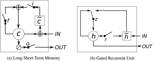
Unlike to the traditional recurrent unit which overwrites its content at each time-step (see Eq.(2)), an LSTM unit is able to decide whether to keep the existing memory via the introduced gates. Intuitively, if the LSTM unit detects an important feature from an input sequence at early stage, it easily carries this information (the existence of the feature) over a long distance, hence, capturing potential long-distance dependencies.
See Fig.1 (a) for the graphical illustration.
|
3.2 Gated Recurrent Unit
A gated recurrent unit (GRU) was proposed by Cho et al. (2014) to make each recurrent unit to adaptively capture dependencies of different time scales. Similarly to the LSTM unit, the GRU has gating units that modulate the flow of information inside the unit, however, without having a separate memory cells.
The activation $h^j_t$ of the GRU at time $t$ is a linear interpolation between the previous activation $h^j_{t−1}$ and the candidate activation $\tilde{h}^j_t$ :
| $h_{t}^{j}=\left(1-z_{t}^{j}\right) h_{t-1}^{j}+z_{t}^{j} \tilde{h}_{t}^{j}$, | (5) |
where an update gate $z^j_t$ decides how much the unit updates its activation, or content. The update gate is computed by
$z_{t}^{j}=\sigma\left(W_{z} \mathbf{x}_{t}+U_{z} \mathbf{h}_{t-1}\right)^{j}$.
This procedure of taking a linear sum between the existing state and the newly computed state is similar to the LSTM unit. The GRU, however, does not have any mechanism to control the degree to which its state is exposed, but exposes the whole state each time.
The candidate activation $\tilde{h}^j_t$ is computed similarly to that of the traditional recurrent unit (see Eq. (2)) and as in Bahdanau et al.(2014),
$\tilde{h}_{t}^{j}=\tanh \left(W \mathbf{x}_{t}+U\left(\mathbf{r}_{t} \odot \mathbf{h}_{t-1}\right)\right)^{j}$ ,
where $r_t$ is a set of reset gates and $\odot$ is an element-wise multiplication[1]. When off ($r^j_t$ close to 0), the reset gate effectively makes the unit act as if it is reading the first symbol of an input sequence, allowing it to forget the previously computed state.
The reset gate $r^j_t$ is computed similarly to the update gate:
$r_{t}^{j}=\sigma\left(W_{r} \mathbf{x}_{t}+U_{r} \mathbf{h}_{t-1}\right)^{j}$.
See Fig. 1 (b) for the graphical illustration of the GRU.
3.3 Discussion
It is easy to notice similarities between the LSTM unit and the GRU from Fig. 1.
The most prominent feature shared between these units is the additive component of their update from $t$ to $t + 1$, which is lacking in the traditional recurrent unit. The traditional recurrent unit always replaces the activation, or the content of a unit with a new value computed from the current input and the previous hidden state. On the other hand, both LSTM unit and GRU keep the existing content and add the new content on top of it (see Eqs. (4) and (5)).
This additive nature has two advantages. First, it is easy for each unit to remember the existence of a specific feature in the input stream for a long series of steps. Any important feature, decided by either the forget gate of the LSTM unit or the update gate of the GRU, will not be overwritten but be maintained as it is.
Second, and perhaps more importantly, this addition effectively creates shortcut paths that bypass multiple temporal steps. These shortcuts allow the error to be back-propagated easily without too quickly vanishing (if the gating unit is nearly saturated at 1) as a result of passing through multiple, bounded nonlinearities, thus reducing the difficulty due to vanishing gradients (Hochreiter, 1991; Bengio et al., 1994).
These two units however have a number of differences as well. One feature of the LSTM unit that is missing from the GRU is the controlled exposure of the memory content. In the LSTM unit, the amount of the memory content that is seen, or used by other units in the network is controlled by the output gate. On the other hand the GRU exposes its full content without any control.
Another difference is in the location of the input gate, or the corresponding reset gate. The LSTM unit computes the new memory content without any separate control of the amount of information flowing from the previous time step. Rather, the LSTM unit controls the amount of the new memory content being added to the memory cell independently from the forget gate. On the other hand, the GRU controls the information flow from the previous activation when computing the new, candidate activation, but does not independently control the amount of the candidate activation being added (the control is tied via the update gate).
From these similarities and differences alone, it is difficult to conclude which types of gating units would perform better in general. Although Bahdanau et al. (2014) reported that these two units performed comparably to each other according to their preliminary experiments on machine translation, it is unclear whether this applies as well to tasks other than machine translation. This motivates us to conduct more thorough empirical comparison between the LSTM unit and the GRU in this paper.
4. Experiments Setting
4.1 Tasks and Datasets
We compare the LSTM unit, GRU and tanh unit in the task of sequence modeling. Sequence modeling aims at learning a probability distribution over sequences, as in Eq.(3), by maximizing the log-likelihood of a model given a set of training sequences:
$\displaystyle \max _{\theta} \frac{1}{N} \sum_{n=1}^{N} \sum_{t=1}^{T_{n}} \log p\left(x_{t}^{n} \mid x_{1}^{n}, \ldots, x_{t-1}^{n} ; \boldsymbol{\theta}\right)$
where $\boldsymbol{\theta}$ is a set of model parameters. More specifically, we evaluate these units in the tasks of polyphonic music modeling and speech signal modeling.
For the polyphonic music modeling, we use three polyphonic music datasets from Boulanger-Lewandowski et al. (2012): Nottingham, JSB Chorales, MuseData and Piano-midi. These datasets contain sequences of which each symbol is respectively a 93 -, 96 -, 105 -, and 108-dimensional binary vector. We use logistic sigmoid function as output units
We use two internal datasets provided by Ubisoft[2] for speech signal modeling. Each sequence is an one-dimensional raw audio signal, and at each time step, we design a recurrent neural network to look at 20 [consecutive samples to predict the following 10 [consecutive samples. We have used two different versions of the dataset: One with sequences of length 500 (Ubisoft A) and the other with sequences of length 8,000 (Ubisoft B). Ubisoft A and Ubisoft B have 7,230 and 800 sequences each. We use mixture of Gaussians with 20 components as output layer.[3]
4.2 Models
For each task, we train three different recurrent neural networks, each having either LSTM units (LSTM-RNN, see Sec. 3.1), GRUs (GRU-RNN, see Sec. 3.2) or tanh units (tanh-RNN, see Eq. (2)). As the primary objective of these experiments is to compare all three units fairly, we choose the size of each model so that each model has approximately the same number of parameters. We intentionally made the models to be small enough in order to avoid overfitting which can easily distract the comparison. This approach of comparing different types of hidden units in neural networks has been done before, for instance, by Gulcehre et al. (2014). See Table 1 for the details of the model sizes.
| Unit | # of Units | # of Parameters |
|---|---|---|
| Polyphonic music modeling | ||
| LSTM | $36$ | $\approx 19.8\times 10^3$ |
| GRU | $46$ | $\approx 20.2\times 10^3$ |
| tanh | $100$ | $\approx 20.1\times 10^3$ |
| Speech signal modeling | ||
| LSTM | $195$ | $\approx 169.1\times 10^3$ |
| GRU | $227$ | $\approx 168.9\times 10^3$ |
| tanh | $400$ | $\approx 168.4\times 10^3$ |
We train each model with RMSProp (see, e.g., Hinton, 2012 and use weight noise with standard deviation fixed to 0.075 Graves, 2011). At every update, we rescale the norm of the gradient to 1, if it is larger than 1 Pascanu et al., 2013 to prevent exploding gradients. We select a learning rate (scalar multiplier in RMSProp) to maximize the validation performance, out of 10 randomly chosen log-uniform candidates sampled from $\mathcal{U}(−12, −6)$ (Bergstra and Bengio, 2012). The validation set is used for early-stop training as well.
5. Results and Analysis
Table 2 lists all the results from our experiments. In the case of the polyphonic music datasets, the GRU-RNN outperformed all the others (LSTM-RNN and tanh-RNN) on all the datasets except for the Nottingham. However, we can see that on these music datasets, all the three models performed closely to each other.
| tanh | GRU | LSTM | |||
|---|---|---|---|---|---|
| Music Datasets | Nottingham | train | 3.22 | 2.79 | 3.08 |
| test | 3.13 | 3.23 | 3.20 | ||
| JSB Chorales | train | 8.82 | 6.94 | 8.15 | |
| test | 9.10 | 8.54 | 8.67 | ||
| MuseData | train | 5.64 | 5.06 | 5.18 | |
| test | 6.23 | 5.99 | 6.23 | ||
| Piano-midi | train | 5.64 | 4.93 | 6.49 | |
| test | 9.03 | 8.82 | 9.03 | ||
| Ubisoft Datasets | Ubisoft dataset A | train | 6.29 | 2.31 | 1.44 |
| test | 6.44 | 3.59 | 2.70 | ||
| Ubisoft dataset B | train | 7.61 | 0.38 | 0.80 | |
| test | 7.62 | 0.88 | 1.26 | ||
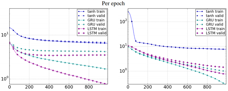
On the other hand, the RNNs with the gating units (GRU-RNN and LSTM-RNN) clearly outperformed the more traditional tanh-RNN on both of the Ubisoft datasets. The LSTM-RNN was best with the Ubisoft A, and with the Ubisoft B, the GRU-RNN performed best.
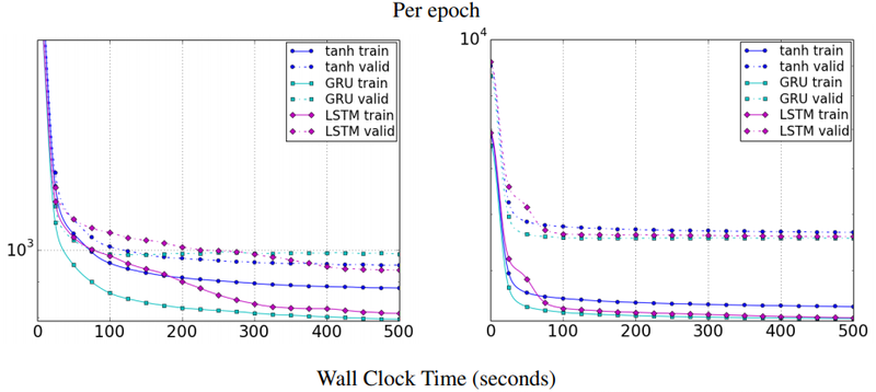
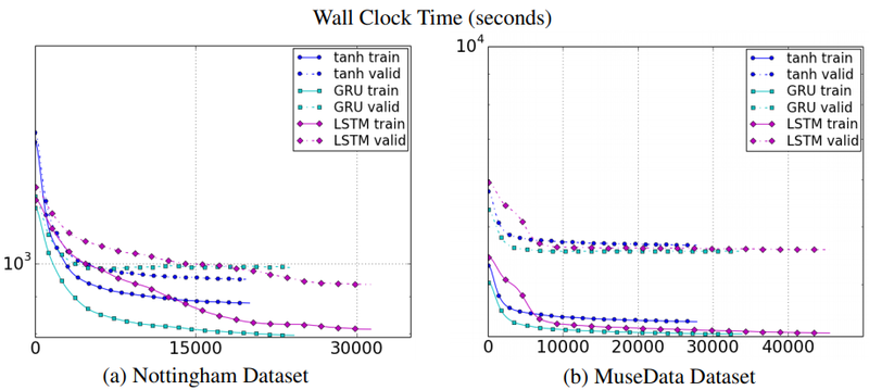
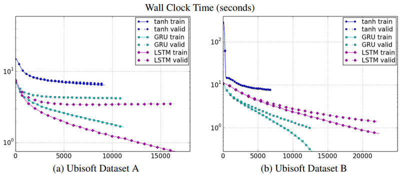
In Figs. 2–3, we show the learning curves of the best validation runs. In the case of the music datasets (Fig. 2), we see that the GRU-RNN makes faster progress in terms of both the number of updates and actual CPU time. If we consider the Ubisoft datasets (Fig. 3), it is clear that although the computational requirement for each update in the tanh-RNN is much smaller than the other models, it did not make much progress each update and eventually stopped making any progress at much worse level.
|
|
|
|
These results clearly indicate the advantages of the gating units over the more traditional recurrent units. Convergence is often faster, and the final solutions tend to be better. However, our results are not conclusive in comparing the LSTM and the GRU, which suggests that the choice of the type of gated recurrent unit may depend heavily on the dataset and corresponding task.
6. Conclusion
In this paper we empirically evaluated recurrent neural networks (RNN) with three widely used recurrent units; (1) a traditional tanh unit, (2) a long short-term memory (LSTM) unit and (3) a recently proposed gated recurrent unit (GRU). Our evaluation focused on the task of sequence modeling on a number of datasets including polyphonic music data and raw speech signal data.
The evaluation clearly demonstrated the superiority of the gated units; both the LSTM unit and GRU, over the traditional tanh unit. This was more evident with the more challenging task of raw speech signal modeling. However, we could not make concrete conclusion on which of the two gating units was better.
We consider the experiments in this paper as preliminary. In order to understand better how a gated unit helps learning and to separate out the contribution of each component, for instance gating units in the LSTM unit or the GRU, of the gating units, more thorough experiments will be required in the future.
Acknowledgments
The authors would like to thank Ubisoft for providing the datasets and for the support. The authors would like to thank the developers of Theano (Bergstra et al., 2010, Bastien et al., 2012) and Pylearn2 (Goodfellow et al., 2013). We acknowledge the support of the following agencies for research funding and computing support: NSERC, Calcul Quebec, Compute Canada, the Canada Research Chairs and CIFAR.
Footnotes
- ↑ 1 Note that we use the reset gate in a slightly different way from the original GRU proposed in Cho et al. (2014). Originally, the candidate activation was computed by$\tilde{h}_{t}^{j}=\tanh \left(W \mathbf{x}_{t}+\mathbf{r}_{t} \odot\left(U \mathbf{h}_{t-1}\right)\right)^{j}$
where $r^j_t$ is a reset gate. We found in our preliminary experiments that both of these formulations performed as well as each other.
- ↑ http://www.ubi.com
- ↑ Our implementation is available at https://github.com/jych/librnn.git
References
2014a
- (Bahdanau et al., 2014) ⇒ Dzmitry Bahdanau, Kyunghyun Cho, and Yoshua Bengio. (2014-2015). “Neural Machine Translation by Jointly Learning to Align and Translate.” In: Proceedings of the Third International Conference on Learning Representations, (ICLR-2015).
2014b
- (Cho et al., 2014) ⇒ Kyunghyun Cho, Bart van Merrienboer, Dzmitry Bahdanau, and Yoshua Bengio. (2014). "On the Properties of Neural Machine Translation: Encoder-Decoder Approaches". In: Proceedings of Eighth Workshop on Syntax, Semantics and Structure in Statistical Translation (SSST@EMNLP 2014). DOI:10.3115/v1/W14-4012
2014c
- (Gulcehre et al., 2014) ⇒ C. Gulcehre, K. Cho, R. Pascanu, and Y. Bengio. Learned-norm pooling for deep feedforward and recurrent neural networks. In Machine Learning and Knowledge Discovery in Databases, pages 530–546. Springer, 2014.
2014d
- (Sutskever et al., 2014) ⇒ Ilya Sutskever, Oriol Vinyals, and Quoc V. Le. (2014). “Sequence to Sequence Learning with Neural Networks.” In: Proceedings of the Advances in Neural Information Processing Systems 27: Annual Conference on Neural Information Processing Systems (NIPS 2014).
2013a
- (Bengio et al., 2013) ⇒ Y. Bengio, N. Boulanger-Lewandowski, and R. Pascanu. Advances in optimizing recurrent networks. In Proc. ICASSP 38, 2013.
2013b
- (Goodfellow et al., 2013) ⇒ I. J. Goodfellow, D. Warde-Farley, P. Lamblin, V. Dumoulin, M. Mirza, R. Pascanu, J. Bergstra, F. Bastien, and Y. Bengio. Pylearn2: a machine learning research library. arXiv preprint arXiv:1308.4214, 2013.
2013c
- (Graves, 2013) ⇒ Alex Graves. (2013). “Generating Sequences With Recurrent Neural Networks.” In: CoRR, abs/1308.0850.
2013d
- (Graves et al., 2013) ⇒ Alex Graves, Abdel-rahman Mohamed, and Geoffrey Hinton. (2013). “Speech Recognition with Deep Recurrent Neural Networks.” In: Proceedings of 2013 International Conference on Acoustics, Speech and Signal Processing (ICASSP 2013). ISBN:978-1-4799-0356-6 doi:10.1109/ICASSP.2013.6638947
2013e
- (Pascanu et al., 2013) ⇒ R. Pascanu, T. Mikolov, and Y. Bengio. On the difficulty of training recurrent neural networks. In: Proceedings of the 30th International Conference on Machine Learning (ICML’13). ACM, 2013. URL http://icml.cc/2013/.
2012a
- (Bastien et al., 2012) ⇒ F. Bastien, P. Lamblin, R. Pascanu, J. Bergstra, I. J. Goodfellow, A. Bergeron, N. Bouchard, and Y. Bengio. Theano: new features and speed improvements. Deep Learning and Unsupervised Feature Learning NIPS 2012 Workshop, 2012.
2012b
- (Bergstra et al., 2012) ⇒ J. Bergstra and Y. Bengio. Random search for hyper-parameter optimization. The Journal of Machine Learning Research, 13(1):281–305, 2012.
2012c
- (Boulanger-Lewandowski et al., 2012) ⇒ N. Boulanger-Lewandowski, Y. Bengio, and P. Vincent. Modeling temporal dependencies in highdimensional sequences: Application to polyphonic music generation and transcription. In: Proceedings of the Twenty-nine International Conference on Machine Learning (ICML’12). ACM, 2012. URL http://icml.cc/discuss/2012/590.html.
2012d
- (Graves, 2012) ⇒ A. Graves. Supervised Sequence Labelling with Recurrent Neural Networks. Studies in Computational Intelligence. Springer, 2012.
2012e
- (Hinton, 2012) ⇒ G. Hinton. Neural networks for machine learning. Coursera, video lectures, 2012.
2011a
- (Graves, 2011) ⇒ A. Graves. Practical variational inference for neural networks. In Advances in Neural Information Processing Systems, pages 2348–2356, 2011.
2011b
- (Martens & Sutskever, 2011) ⇒ J. Martens and I. Sutskever. Learning recurrent neural networks with Hessian-free optimization. In Proc. ICML’2011. ACM, 2011.
2010
- (Bergstra et al., 2010) ⇒ J. Bergstra, O. Breuleux, F. Bastien, P. Lamblin, R. Pascanu, G. Desjardins, J. Turian, D. WardeFarley, and Y. Bengio. Theano: a CPU and GPU math expression compiler. In: Proceedings of the Python for Scientific Computing Conference (SciPy), June 2010. Oral Presentation.
1997
- (Hochreiter & Schmidhuber, 1997) ⇒ S. Hochreiter and J. Schmidhuber. Long short-term memory. Neural Computation, 9(8):1735–1780, 1997.
1994
- (Bengio et al., 1994) ⇒ Y. Bengio, P. Simard, and P. Frasconi. Learning long-term dependencies with gradient descent is difficult. IEEE Transactions on Neural Networks, 5(2):157–166, 1994.
1991
- (Hochreiter, 1991) ⇒ S. Hochreiter. Untersuchungen zu dynamischen neuronalen Netzen. Diploma thesis, Institut fur¨ Informatik, Lehrstuhl Prof. Brauer, Technische Universitat M ¨ unchen, 1991. URL ¨ http:// www7.informatik.tu-muenchen.de/˜Ehochreit.
BibTeX
@article{2014_EmpiricalEvaluationofGatedRecur,
  author    = {Junyoung Chung and
               Caglar Gulcehre and
               KyungHyun Cho and
               Yoshua Bengio},
  title     = {Empirical Evaluation of Gated Recurrent Neural Networks on Sequence
               Modeling},
  journal   = {CoRR},
  volume    = {abs/1412.3555},
  year      = {2014},
  url       = {http://arxiv.org/abs/1412.3555},
  archivePrefix = {arXiv},
  eprint    = {1412.3555},
}
| Author | volume | Date Value | title | type | journal | titleUrl | doi | note | year | |
|---|---|---|---|---|---|---|---|---|---|---|
| 2014 EmpiricalEvaluationofGatedRecur | Yoshua Bengio Alex Graves Caglar Gulcehre Junyoung Chung KyungHyun Cho | Empirical Evaluation of Gated Recurrent Neural Networks on Sequence Modeling | 2013 2014 |